


 Extract (6-MSITC) in Healthy Older Adults")
: An In-Depth Exploration into its Thermogenic Role and Social Significance")


A new map of the mountains, valleys and canyons hidden under Antarctica’s ice has revealed the deepest land on Earth, and will help forecast future ice loss.
The frozen southern continent can look pretty flat and featureless from above.
But beneath the ice pack that’s accumulated over the eons, there’s an ancient continent, as textured as any other.
And that texture turns out to be very important for predicting how and when ice will flow and which regions of ice are most vulnerable in a warming world.
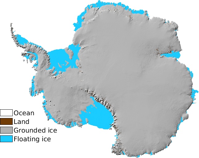
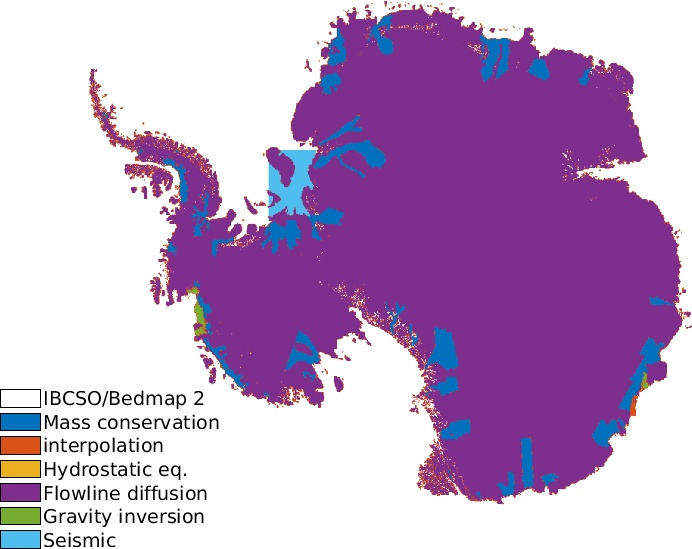
The new NASA map, called BedMachine Antarctica, mixes ice movement measurements, seismic measurements, radar and other data points to create the most detailed picture yet of Antarctica’s hidden features.
“Using BedMachine to zoom into particular sectors of Antarctica, you find essential details, such as bumps and hollows beneath the ice that may accelerate, slow down or even stop the retreat of glaciers,” Mathieu Morlighem, an Earth system scientist at the University of California, Irvine and the lead author of a new paper about the map, said in a statement.
The new map, published Dec. 12 in the journal Nature Geoscience, reveals previously unknown topographical features that shape ice flow on the frozen continent.
The previously unknown features have “major implications for glacier response to climate change,” the authors wrote.
“For example, glaciers flowing across the Transantarctic Mountains are protected by broad, stabilizing ridges.”
Understanding how ice flows in Antarctica becomes increasingly important as Earth warms.
If all of Antarctica’s ice were to melt, it would raise global sea levels by 200 feet (60 meters), according to the National Snow and Ice Data Center.
That isn’t likely anytime soon, but even if small fractions of the continent were to melt, it would have devastating global effects.
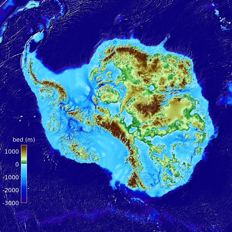
Included in the data is evidence for the deepest canyon on planet Earth.
By studying how much ice flows through a particular, narrow region known as the Denman trough each year, the researchers realized it must dive at least 11,000 feet (3,500 meters) below sea level to accommodate all the frozen water volume.
That’s far deeper than the Dead Sea, the lowest exposed region of land, which sits 432 meters (1,419 feet) below sea level, according to the Israel Oceanographic and Limnological Research center.
The map offers a wealth of new information on precisely which regions of the continent’s ice are at most risk of sliding into the ocean in the coming decades and centuries, the authors wrote.
BedMachine Antarctica
Since 2014, we have been working on a self-consistent dataset of the Antarctic Ice Sheet based on the conservation of mass that is now freely available at NSIDC.
Note: keep in mind that not all of the bed is mapped using mass conservation (MC). If there is a fast flowing region that is currently not mapped with MC, let me know and I will try to add it in the next release. If you have ice thickness data that is not included, I would also be more than happy to add it to the mapping to further improve the topography.
Description
The data are in one single file in NetCDF format (795 Mb) and all heights are in meters above mean sea level (the geoid used is provided in the NetCDF file). All the data use the same 450 m-resolution grid although the “true” resolution of the bedrock may vary depending on the method used to map the bed. This dataset uses data from 1993 to 2016 and has a nominal date of 2012 (same as REMA).
For the hydrostatic equilibrium calculation, we used a density of ice ρice=917 kg/m3, and an ocean water density of ρocean=1027 kg/m3 (following the densities used in Griggs & Bamber 2011 and Chuter & Bamber 2015).
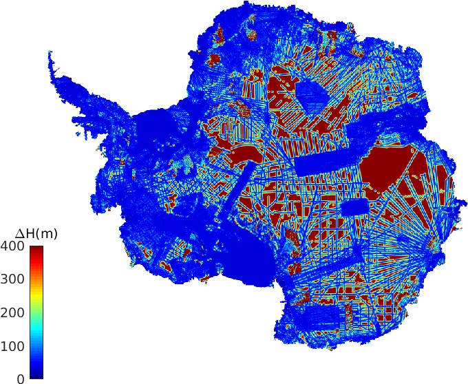
As any model output, there are errors in these maps (there is an estimate included in the dataset). Feedback is more than welcome.
Citation
Morlighem, M., Rignot, E., Binder, T. et al. Deep glacial troughs and stabilizing ridges unveiled beneath the margins of the Antarctic ice sheet. Nat. Geosci. (2019) doi:10.1038/s41561-019-0510-8
Disclaimer
The ice thickness and bed topography are model outputs and are not free of error (especially in regions where ice thickness measurements are sparse). This dataset is a work in progress and we encourage users to send us feedback so that we keep improving it.
Projection
The projection is Polar Stereographic South (71ºS, 0ºE), which corresponds to ESPG 3031
Reading with MATLAB
MATLAB now has an extensive library for NetCDF files.
filename = 'BedMachineAntarctica-2019-09-04.nc';
x = ncread(filename,'x');
y = ncread(filename,'y');
bed = ncread(filename,'bed')'; %Do not forget to transpose (MATLAB is column oriented)
%Display bed elevation
imagesc(x,y,bed); axis xy equal; caxis([-1000 3000]);
Converting heights to WGS84
All heights are referenced to mean sea level (using the geoid EIGEN-6C4). To convert the heights to heights referenced to the WGS84 ellipsoid, simply add the geoid height:
zellipsoid=zgeoid+geoid
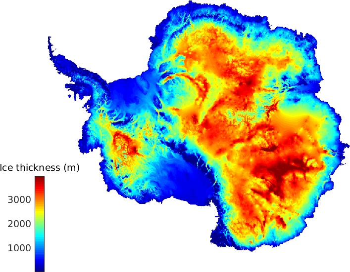
Surface height and firn depth correction
All the quantities provided in BedMachine are in ice equivalent. This affects primarily the upper surface of the ice, to which we have subtracted a firn depth correction to account for the presence of air in the firn layer. The ice thickness is also in ice equivalent. To recover the top of the surface dem from RAME in WGS84:
zREMA=surface+firn+geoid
where “firn” is the firn depth correction, “surface” is the surface height, and “geoid” is the geoid height. All these quantities are provided in the netCDF file.


