How much are you conscious of right now?

How much are you conscious of right now?

Are you conscious of just the words in the centre of your visual field or all the words surrounding it?

We tend to assume that our visual consciousness gives us a rich and detailed picture of the entire scene in front of us.

The truth is very different, as our discovery of a visual illusion, published in Psychological Science, shows.

To illustrate how limited the information in our visual field is, get a deck of playing cards. Pick a spot on the wall in front of you and stare at it.

Then take a card at random. Without looking at its front, hold it far out to your left with a straight arm, until it’s on the very edge of your visual field. Keep staring at the point on the wall and flip the card round so it’s facing you.

Try to guess its colour. You will probably find it extremely difficult. Now slowly move the card closer to the centre of your vision, while keeping your arm straight. Pay close attention to the point at which you can identify its colour.

It’s amazing how central the card needs to be before you’re able to do this, let alone identify its suit or value. What this little experiment shows is how undetailed (and often inaccurate) our conscious vision is, especially outside the centre of our visual field.

Crowding: how the brain gets confused

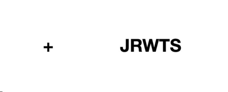
Here is another example that brings us a little closer to how these phenomena are investigated scientifically. Please focus your eyes on the + sign on the left, and try to identify the letter on the right of it (of course you know already what it is, but pretend for the moment that you do not):

You might find this a bit tricky, but you can probably still identify the letter as an “A”. But now focus your eyes on the following +, and try to identify the letters on the right:

In this case, you’ll probably struggle to identify the letters. It probably looks like a mess of features to you. Or maybe you feel like you can see a jumble of curves and lines, without being able to say precisely what’s there.

This is called “crowding”. Our visual system sometimes does OK at identifying objects in our peripheral vision, but when those objects are placed near other objects, it struggles. This is a shocking limitation on our conscious vision. The letters are clearly presented right in front of us. But still our conscious mind gets confused.

Crowding is a hotly debated topic in philosophy, psychology and neuroscience. We’re still not sure why crowding happens. One popular theory is that it’s a failure of what’s called “feature integration”. To understand feature integration, we will need to pick apart some of the jobs that your visual system does.

Imagine you are looking at a blue square and a red circle. Your visual system does not just have to detect the properties out there (blueness, redness, circularity, squareness).

It also has to work out which property belongs to which object. This might not seem like a complicated task to us. However, in the visual brain, this is no trivial matter.

It takes a lot of complicated computation to work out that circularity and redness are properties of one object at the same location. The visual system needs to “glue” together the circularity and the redness as both belonging to the same object, and do the same with blueness and squareness. This gluing process is feature integration.

According to this theory, what happens in crowding is that the visual system detects the properties out there, but it can’t work out which properties belong to which object. As a result, what you see is a big mess of features, and your conscious mind cannot differentiate one letter from the others.

New illusion

Recently, we have discovered a new visual illusion that has raised a host of new questions for fans of crowding. We tested what happens when three of the objects are identical, for example in the following case:

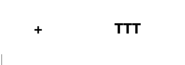
What do you see when you look at the +? We found that more than half of people said that there were only two letters there, rather than three. Indeed, follow-up work seems to indicate that they’re pretty confident about this incorrect judgment.

This is a surprising result. Unlike normal crowding, it’s not that you see a jumble of features. Rather, one whole letter neatly drops away from consciousness.

This result fits poorly with the feature integration theory. It’s not that the visual system is detecting all of the properties out there, but just getting confused about which properties belong to which objects. Rather, one whole object has just disappeared.

We don’t think that a failure of feature integration is what’s going on. Our theory is that this illusion is due to what we call “redundancy masking”. In our view, the visual system can detect that there are several of the same letter out there, but it doesn’t seem to calculate correctly how many there are. Maybe it’s just not worth the energy to work out the number of letters with high precision.

When we open our eyes, we effortlessly get a conscious picture of our environment. However, the underlying processes that go into creating this picture are anything but effortless. Illusions like redundancy masking help us unpick how these processes work, and ultimately will help us explain consciousness itself.

Funding: Bilge Sayim receives funding from the French Agence Nationale de la Recherche (ANR), I-SITE ULNE, and the Swiss National Science Foundation (SNSF).

Henry Taylor does not work for, consult, own shares in or receive funding from any company or organization that would benefit from this article, and has disclosed no relevant affiliations beyond their academic appointment.

---

In 1962, the ophthalmologists James Stuart and Hermann Burian published a study on amblyopia where they adopted a nice and clear term when they spoke of the crowding phenomenon1,2 to describe why standard acuity test charts are mostly unsuitable for amblyopic subjects: On most standard charts, as ophthalmologists and optometrists knew, optotypes on a line are too closely spaced for valid assessment of acuity in all cases such that in particular amblyopic subjects (and young children) may receive too low an acuity score.

The phenomenon had been reported briefly earlier by the Danish ophthalmologist Holger Ehlers3 (Ehlers, 1936, 1953), who was perhaps the first to use the term crowding in that context, and it was treated in Adler’s textbook (Adler, 1959, pp. 661–662). Because amblyopic vision—commonly known as the “lazy eye syndrome”—leads to a strangely impaired percept and is quite unlike familiar blurred vision, it has, for the purpose of illustration, often been likened to peripheral (or indirect4) vision, which shares that obscurity (Strasburger & Wade, 2015a).

Indeed, the same phenomenon of crowding with closely spaced patterns occurs there, that is, at a few degrees of visual angle away from where one fixates. A simple example is shown in Figure 1. Viewed at arm length, the left duck is at very roughly 4° eccentricity, and, when surrounded by fellow ducks, the same duck at the right and the same eccentricity is indistinct and obscure.

Note that the visibility is not a matter of the target size here, that is, it has nothing to do with acuity or resolution in the visual field. Note further that standard textbook theories based on local, bottom-up processing, invoking simple versus complex receptive field types, retinal lateral inhibition, rate of convergence/divergence of sensory neurons, and the like, will not explain the phenomenon that, as we today know, happens in the cortex (for discussions of theories see, e.g., Tyler & Likova, 2007; Pelli, 2008; Strasburger, 2014; Kwon et al., 2014; Rosenholtz, 2015; Strasburger, 2019). Simple as it is, this little demonstration—by its ubiquity in everyday natural scenes, and its simplicity (it can be shown on a napkin)—already shows that we have a very basic, general phenomenon of visual perception here, not some niche interest of vision researchers.

Independently, and at around the same time, the phenomenon and related phenomena were studied quite extensively in a separate research tradition, Gestalt psychology (Korte, 1923) and later in experimental psychology (e.g. Wolford, 1975; Krumhansl & Thomas, 1977; Chastain, 1982, 1983).

Little did these two research communities appear to know of each other: By the time that I started being interested in crowding in 1988, there were 20 major articles on the subject, under a variety of keywords (lateral masking/inhibition/interference, interaction effects, contour interaction, surround suppression), which, more often than not, took scarce notice of those of the other line of thought (as evidenced by their references).

There were only few articles at vision conferences and none in the emerging cognitive sciences or in visual neuroscience.

Things changed in the 1990s and early 2000s. Levi et al. (1985) had studied crowding in vernier acuity; Lewis O. Harvey suggested that we (myself, Ingo Rentschler, and Lew Harvey) study character crowding at low contrast and ask what mechanisms might underlie crowding (Strasburger et al., 1991; Strasburger & Rentschler, 1995).

Latham and Whitaker (1996) studied the influence of four surrounding flankers on a three-bar grating, where they showed that spatial interference grew at a much faster rate with eccentricity than acuity (with E2 values5 only one tenth of those for acuity). He et al. (1996) pointed to the role of spatial attention, and, in particular, Denis Pelli started projects on crowding6 and, together with Melanie Palomares and Najib Majaj, published a seminal article, covering all the basics (Pelli et al., 2004).

Crucially, however, Pelli drew attention to the fact that, contrary to common wisdom, crowding is much more important for pattern recognition than is acuity and that it overrides the latter even in the fovea,7 widely held to be superior because of its outstanding acuity in its centre (Latham & Whitaker, 1996; Pelli et al., 2007; Pelli & Tillman, 2008).

Small as it might seem, the shift of emphasis away from (inherently low-level) acuity to (inherently higher level) crowding amounts, as I see it, to nothing less than a paradigm shift. It does away with centuries of two core assumptions in visual perception (cf. Strasburger & Wade, 2015a), namely that good vision comes down to good acuity and, more generally, that a reductionist approach is necessarily and always the best way for solving a scientific problem.

The acuity myth is everywhere. We find it in driving licence regulations (where acuity tests are often the only strict psychometric requirement for a driver’s license), or when a textbook presents a trivialized dichotomy of parvo (P) and magno (M) systems in which the P system is supposedly specialized on pattern recognition because of its high resolution and small receptive fields.

Thomas Kuhn in The Structure of Scientific Revolutions (Kuhn, 1962) explains that research traditions in science often pervade through many decades (or perhaps centuries?), adding more and more detail to a scientific narrative until suddenly, within a few years, the viewpoint shifts radically and something new starts. The shift of emphasis in human and primate pattern recognition from acuity to crowding might just represent such a turn.

Perception is a standard, and often required, subject in psychology, medicine, and other curricula, and so there are quite a few excellent textbooks on perception and on the senses. A standard for covering all the senses, for example, is Goldstein’s well-known Sensation and Perception.

Acuity, receptive fields, cortical magnification, and peripheral vision are all covered—yet it says nothing about crowding. Even more worrying, acuity and crowding are confused as shown in Figure 2. The lapse might be excused in that vision is not the author’s primary field of study.

But that explanation does not transfer to the several German editions, which were edited by expert vision scientists (e.g., 7th German edition, 2008, p. 50). Another standard, Basic Vision by Snowden et al. (2006), a more recent, and excellent perception textbook for the visual modality, explains cortical magnification and shows Anstis’s visual demonstration of that in its first edition but also skips crowding. The same is the case in the new, 2nd edition (2012).

The section on peripheral vision (pp. 117–119) shows a modified version of Anstis’s magnification chart and explains scaling and cortical magnification (the chart is the impressive but misleading version of Figure 9B discussed later here in the article, with a caption8 that warrants understanding why it is wrong).

Mind you, the examples mentioned are already the positive exceptions. Peripheral vision and crowding are the poor relations in vision research.

Out of 20 textbooks on vision that I went through published between 1970 and 2019, only 5 had some rudimentary coverage of peripheral vision (though without a term in the index), and even fewer mentioned crowding (three). The others, including the monumental, 1,800-page Visual Neurosciences by Chalupa and Werner (2004), the excellent and beautifully designed new Sensation and Perception by Yantis and Abrams (2017), and seven textbooks on computational vision, are silent on the subjects. The venerable Sekuler and Blake (1994), Perception, in contrast, and the brand new Sensation & Perception by Wolfe et al. (2019) have it right. Sekuler and Blake show and discuss Anstis’s charts on peripheral vision and crowding (see Figure 9), and Wolfe et al. (pp. 43–45) explain peripheral vision and show the well-known graph on receptor density (originally by Oesterberg, 1935), and explain crowding (p. 76) with reference to a figure from Whitney and Levi (2011).

Thus, either crowding is, after all, much less important for vision in general than those who work on that subject believe it is or now is the time that crowding will enter our textbooks and curricula. The frequent publications, talks, and symposia at vision conferences, the workshops,9 theses, and in short the observation that crowding is nowadays a kind of vision-research household item would suggest the latter.

In that case, it matters that in the sudden flood of interest, quite a number of misconceptions on the topic appear to arise. To ensure, therefore, that these are kept at bay (or do not arise in the first place)—in particular in the perception books that are to come—here is an attempt to pinpoint a number of beliefs, or intuitive theories (Lucariello & Naff, 2019),10 that, upon more scrutiny, turn out to be misleading or perhaps just wrong. Note this is not about finding erroneous beliefs in the crowding literature; authors in the field rarely fall for these errors.

The point is how, eventually, the key concepts for crowding will come across in, say, a textbook chapter, with its inherent need for brevity and graphicness. Assertions that seem unambiguous can turn out to be obstacles for understanding. Nota bene, the seven points are also not all of the same quality; they range from possible misunderstandings, questionable assertions, and apparent misconceptions, to clear-cut myths.

Their selection reflects what I found interesting and noteworthy. Note also that, for now, the following is mostly about the isolated, “standard” crowding task—a target with singly occurring flankers. It is not about visual crowding (or crowding theories) in general.

There will thus be further issues that might qualify as “myths,” like the hope that two mechanisms might eventually be specified that explain crowding (many authors including myself invoke two mechanisms; they are just rarely the same). I simply stopped after seven points. The article is the sixth in a series of—slightly pointed—“myths” presentations in vision research that I am aware of (Wade & Tatler, 2009; Rosenholtz, 2016; Bach, 2017; Strasburger, 2017a, 2017b, 2018), and I trust more will follow.11

Interestingly, there is no catchy German word for crowding, and so the English term has entered German-language scientific writing. Conversely (and on the light side), the German germane wimmelbild (wimmeln = to swarm with) is sometimes seen on English pages instead of the “Find Waldo”/“Where’s Wally” catch phrases, and in any case, those crowded images are about to develop into an art form of their own (Figure 3).

On Bouma’s Law
Misconception 1: Bouma’s law can be summarized, succinctly and unequivocally, as saying that “critical distance for crowding is about half the target’s eccentricity, d≈0.5 φ (Bouma, 1970).”

In a sense that is of course correct: Bouma’s law is based on an experiment on letter triplets described in a Nature paper by Bouma (1970); it governs how crowding depends on the flankers’ distance to the target and specifies the minimum distance for the interference as being approximately half the eccentricity value.

It operates over at least a hundredfold range. However, the simplicity of the above statement’s phrasing and the attribution are deceptive and can give rise to a number of misunderstandings.

Three of these I wish to address here:

• (a) the law’s generality and the role of Gestalt mechanisms;
• (b) whether critical distance can be seen as a critical window, and (as the main point here),
• (c) what is meant by the word “about,” the role of a constant term, and what constitutes a law.

On the first point, Bouma’s finding turned out amazingly robust and general in describing a large variety of basic crowding situations; it works with letters, low-contrast numerals, Landolt rings, gratings, and many other patterns, and amid many kinds of flankers in various numbers and orientations. It further tells us a lot about recognition of more complex patterns.

After its first confirmation (Strasburger et al., 1991), Pelli et al. (2004) have studied a wide range of conditions and were the first to refer to it as Bouma’s rule (p. 1143). A few years later, Pelli and Tillman (2008) discussed findings on its generality for proposing to raise Bouma’s (1970) rule of thumb12 to the rank of a law. Yet in spite of that impressive range of applicability, it needs to be remembered that Bouma’s law is not a descriptor for crowding in general.

The reason for this is that human pattern recognition (see, e.g., Strasburger et al., 2011; DiCarlo et al., 2012), for which the crowding phenomenon is a central ingredient, can be subject to Gestalt mechanisms (it is worth rereading Korte, 1923, here to remind oneself of the phenomenology).

Gestalt mechanisms can have the opposite effects of crowding and override the specifics of local stimulus configurations, as in the examples cited later, obeying the simple truth that the whole is generally more than the sum of its parts. So as indicated in the Introduction section, the proven and tested concept of simplifying by analytical dissection can lead astray, in particular for the case of crowding, as the isolated crowding stimulus configurations like the one in Figure 1 or Figure 4A (further below) do not predict target recognition when embedded in a larger surround.

A typical Gestalt mechanism is grouping, by which the interference of the flankers in crowding can be eliminated or even inversed by adding a background with which those flankers group. This has been shown first by Banks et al. (1979, Figure 5) and Wolford and Chambers (1983, Figure 1) (see Herzog & Manassi, 2015, Figure 2A, and Strasburger et al., 2011, Figure 19, respectively).

More recently, it has been explored systematically in Bonneh and Sagi (1999), Levi and Carney (2009), Livne and Sagi (2007, 2010), and in a series of studies by Michael Herzog and coworkers (Malania et al., 2007; Sayim et al., 2008, 2010; Saarela et al., 2009; Manassi et al., 2012, 2013; Herzog et al., 2015; see Herzog & Manassi, 2015, for review).

Their message can be summarized as saying that “appearance (i.e., how stimuli look) is a good predictor for crowding” (Herzog et al., 2015, p. 1). Chakravarthi and Pelli (2011) give that view a twist in saying it is not grouping among flankers that reduces crowding but, instead, that crowding is mediated by grouping of the flankers with the target (and is unaffected by grouping of the flankers with each other).

That said, this does not mean that, when grouping is involved, the distance between target and flankers no longer matters. All things equal, larger distance still means less crowding. The dependence on distance is changed, however, and in complicated ways that are not yet understood. Thus, grouping does not necessarily invalidate Bouma’s law; it rather challenges us clarifying how Gestalt mechanisms interact with the local situation and thereby modify Bouma’s law.

A second case in point concerns the influence of flankers further away than the critical distance and is related to the concept of a crowding window, introduced by Pelli in 2008 (Pelli, 2008; Pelli & Tillman, 2008). The proposed concept of a crowding window implies that crowding would occur only below the critical distance. Indeed, Pelli et al. (2004, p. 1146) suggested earlier that additional flankers on the left and right have little or no influence (they point out, however, that the data of Strasburger et al. (1991) contradict that assumption).

Herzog and Manassi (2015, p. 86), in that context, phrase “Bouma (1970) showed that […] flankers interfere only when presented within a critical window […] (Bouma’s law).” That can still be read in two ways: as talking about Bouma’s original two-flanker task (for which it would be correct), (the qualifier only would then refer to the tested flanker distances), or as ruling out influences from outside the window (where the qualifier only refers to the closest vs. other flankers). However, Herzog et al. (2015, p. 1) phrase the assertion explicitly as “Crowding is determined only by nearby elements within a restricted region around the target (Bouma’s law).”

That is, by the citation, the nearest-flanker-only rule is considered part of Bouma’s law. Both articles continue to show that the assertion of no influence from outside the window is incorrect and thus appears to disprove Bouma’s law (Strasburger et al., 1991, had already shown that four flankers on the horizontal meridian exert more influence than two, that is, that the assertion of no influence from outside is incorrect).

Now, given that Bouma himself never talked about a multiple-flanker crowding situation and, further, that the evidence is clearly against a “nearest-only” assertion, it would seem that this assertion should not be made a constituent for a law in Bouma’s name. We thus need to pay close attention to the law’s precise phrasing and to the referenced attribution.

As to the idea of a crowding window where only the nearest neighbour counts, another interesting example for why the exact wording of Bouma’s rule (or law) matters is the article by Van der Burg et al. (2017, p. 690) on the applicability of Bouma’s rule (or law) in large, cluttered displays.

The article argues that, “If visual crowding in dense displays is [not] subject to Bouma’s law, then this questions the fundamental applicability of Bouma’s law in densely cluttered displays.” (p. 693). Its conclusion is “that Bouma’s rule does not necessarily hold in densely cluttered displays [and] instead, a nearest-neighbour segmentation rule provides a better account.” (p. 690). Again, this is about disproving.

On the surface, this might be taken as saying that Bouma’s law as expressed in Equation 1 or 2 does not hold when displays are complex. But this is not at all what is meant in that article. What is meant (but not said in the summary) is simply that the half-eccentricity rule was not met at the specific tested eccentricity, and this, as a counterexample, disproves the generality of the rule (remember, in mathematics a single counterexample disproves a law).

Only a single eccentricity was tested (because the article’s goal was elsewhere), so linearity or the dependence on eccentricity were not at stake. The results would be compatible, for example, with Bouma’s rule as stated in Pelli et al. (2004), just with a much smaller slope factor. So again, when a rule is disproven, it is imperative to behold the precise phrasing that is referred to (in this case the original rule).

As to the third of the points listed earlier, what follows here in the article is about the isolated crowding task. For that, the statement in the header sounds sensible enough and suffices as a rule of thumb, as originally intended. We can do better, however. The amazing robustness and generality across configurations of that rule suggests there is something much more fundamental about it.

Starting with Pelli et al. (2007) and Pelli (2008), and in particular its discussion by Pelli and Tillman (2008), authors now frequently (and with good reason) consider it a law rather than a mere rule of thumb, equal in rank to other laws of psychophysics like Weber’s law, Riccò’s law, Bloch’s law, and so forth. Now the requirements for a law as, for example, standardly applied in classical physics are higher. One requirement is generality, but this is obviously a given, at least for the isolated crowding task.

Another requirement, however, concerns the mathematical formulation. Not only should the mathematical description of a real-world dependency fit the empirical data, it must crucially also fulfil certain a-priori, theoretical constraints: namely to make sense for the obvious cases.

That is, it must obey boundary conditions. As a trivial example, in the equation specifying the distance of the earth to the moon in the elliptical orbit, that distance may vary, but it must not be negative, and better not be zero. Or, for Weber’s law, zero intensity must be excluded for the principled reason that Weber’s ratio is undefined there (and the law further breaks down near the absolute threshold as explained by a statistical model by Barlow, 1957). Riccò’s law must be constrained to the area in which energy summation takes place, and so forth. A lack of such constraints is where the mathematical formulation in the header fails.

To get to that point, let us consider the qualifier about in the header statement. Mostly, it is understood as referring to the factor 0.5 in Bouma’s equation: d=0.5 φ(1) where d is critical distance—the minimum distance between target and flanker below which crowding occurs—and φ is eccentricity in degrees visual angle. Whitney and Levi (2011), in their discussion whether Bouma’s rule would qualify as a law, find the dependency of that factor on multiple influences the main issue that speaks against a law.

Indeed, that factor may vary quite a bit between tasks, roughly between 0.3 and 0.7, as Pelli et al. (2004, Table 4) have listed up in their review of tasks, sometimes much more (between 0.13 and 0.713 in Strasburger and Malania, 2013, Figure 9A). Linearity, in contrast, holds amazingly well for almost all visual tasks.14 So while there is ambiguity about the factor, that ambiguity can be easily accounted for by replacing the fixed slope factor of 0.5 in the equation by a parameter that depends on the respective task in question.

There is a more important slur, however, a limitation of the rule’s generality in range. This becomes apparent when considering the particularly important case for crowding: foveal vision and reading. The eccentricity angles (φ) in question are small there, and thus the precise meaning of a critical distance becomes important (Figure 4). Bouma (1970) specified d as the threshold of internal or empty space between target and flankers;15 today’s authors mostly prefer to specify flanker distance as measured centre-to-centre, as critical spacing then remains mostly constant across sizes as has often been shown (Tripathy & Cavanagh, 2002; Pelli et al., 2004; Pelli & Tillman, 2008; Levi & Carney, 2009; Coates & Levi, 2014; cf. also van den Berg et al., 2007, even though the independence is not perfect, e.g., Gurnsey et al., 2011).

At small eccentricities, where (by Bouma’s rule) flankers at the critical distance are close to the target, that difference of specification matters (Figure 5). With Bouma’s empty-space definition, critical distance is proportional to eccentricity (pink line in Figure 5A, going through the origin). With the centre-to-centre definition, in contrast, critical distance is not proportional to eccentricity; it is just a little bigger, by one-letter width.

The difference is seen in Figure 5A, where the blue line is shifted vertically relative to the pink line. The blue line has a positive axis intercept and represents a linear law, not proportionality. With the centre-to-centre definition in Equation 1, the stimulus configuration would become meaningless in the fovea centre: Proportionality would imply that target and flankers are at the identical location in the centre; just off the centre, target and flankers would overlap, as shown in Figure 5B. Importantly, it is not what Bouma said.

To sum up the third point, in today’s terminology, Bouma described a linear law, not proportionality:

d=0.5 φ+w(2)

where w is letter width.16 We warned against this fallacy before (e.g., Strasburger et al., 2011, p. 34). Notably, Weymouth (1958) had already pointed out the importance of that difference.

Yet perhaps Equation 1 is just more elegant and appealing. Note then that Equation 2 is formally equivalent to M scaling (i.e., compensating for the differing cortical neural machinery across the visual field). Isn’t that beautiful? It has ramifications of its own that we wrote about elsewhere (Strasburger & Malania, 2013; Strasburger, 2019; for a review of M scaling, see Strasburger et al., 2011, Section 3, or Equation 9, below, and Schira et al., 2009, 2010). We will get back to that towards the end of the article, when we speak about the cortical map.

Crowding and Peripheral Vision
Misconception 2: Crowding is predominantly a peripheral phenomenon.

Crowding is of course highly important in the visual periphery. It is often even said to be the characteristic of peripheral vision (e.g., when amblyopic vision is likened to peripheral vision).

Yet—and that is mostly overlooked—in a sense, crowding is even more important in the fovea. There, it is the bottleneck for reading and pattern recognition. Pelli and coworkers have pointed that out most explicitly (Pelli et al., 2007; Pelli & Tillman, 2008).

Beware in that context that the fovea is much larger than one is mostly aware of: Its diameter is standardly stated to be around 5° visual angle (Polyak, 1941;17 Wandell, 1995). Note also that ophthalmologists appear to use the terms differently, referring to the 5° diameter area as the macula lutea even though the anatomical macula is again larger (diameter 6°–10°,18 or 17° following Polyak, 1941).

Another source of confusion is the use of the term foveal vision. When vision scientists use that term, or speak of “the fovea,” they are typically not referring to the foveal area but are talking about the situation where the observer fixates; that is, they effectively refer to the foveola (having about 1.4° diameter following Polyak, 1941, or 0.5° diameter for a completely rod-free area; Tyler & Hamer, 1990).

Or, indeed, they might refer to the point of highest receptor density, the very centre, sometimes called the foveal bouquet (Oesterberg, 1935; Polyak, 1941; Tyler & Hamer, 1990). That maximum is reached in an area of only about 8 to 16 arcmin diameter (Li et al., 2010, Figure 619). The actual point of fixation (i.e., the preferred retinal locus) is furthermore not there but is between 0 and 15 arcmin away from that point (Li et al., 2010, Table 2).

As a practical example, when an optometrist or ophthalmologist measures visual acuity, the result likely refers to the short moment when the gap of the Landolt ring is at the preferred retinal locus, that is, it is likely several arcmin away from the fovea’s centre. It is then that maximum acuity is achieved, and in young adults, roughly two thirds of a minute of arc are resolved at good illumination (Frisén & Frisén, 1981).

In the rest of the fovea, acuity as we all know is much lower. Phrased a bit offhand, resolving Landolt gaps is not of foremost interest for reading: Letter sizes in normal reading far exceed the acuity limit. In normal reading, letter size is somewhere around 0.4 to 2 degrees (Legge et al., 1985; Pelli et al., 2007, Figure 1)—5 to 25 times the 20/20 acuity limit.

Within the fovea, crowding is not only present off-centre (i.e., for indirect vision) but is also present in the very centre. This is what is meant by the term foveal crowding. Its presence has been controversial for a time but appears now well established (Flom et al., 1963; Loomis, 1978; Jacobs, 1979; Levi et al., 1985; Nazir, 1992; Polat & Sagi, 1993, 1994; Levi et al., 2002a; Ehrt & Hess, 2005; Danilova & Bondarko, 2007; Sayim et al., 2008, 2010; Lev et al., 2014; Coates & Levi, 2014; Siderovet al., 2014; Coates et al., 2018; for short reviews, see Loomis, 1978; Danilova & Bondarko, 2007; Lev et al., 2014; Coates & Levi, 2014; Coates et al., 2018). There is agreement that the interaction effect of foveal acuity targets, measured with conventional techniques, occurs “within a fixed angular zone of a few min arc” (3’–6’; Siderov et al., 2013, 2014, p. 147). However, a new study using adaptive optics (Coates et al., 2018) shows critical spacings are indeed even much smaller and only about a quarter of that range, 0.75 to 1.3 arcminutes edge-to-edge.

Whether the lateral interactions in the centre should be called “crowding” is another question. Its characteristics might (or might not) be different from those further out. Levi et al. (2002b) have it in the title—“Foveal crowding is simple contrast masking.”

Coates and Levi (2014) and Siderov et al. (2014) consequently—like Flom et al. (1963)—speak of contour interaction. Namely, whereas crowding appears to be mostly independent of letter size (Strasburger et al., 1991; Pelli et al., 2004), that seems less so to be the case for the fovea centre, and is described by Coates and Levi (2014) as conforming with a two-mechanism model in which the critical spacing for foveal contour interaction is fixed for S < 5’ and proportional to target size for S > 5’ (Figure 6A and B).

Coates and Levi (2014) call that behaviour the hockey stick model. Yet the new adaptive-optics data show that, for small sizes and if suitably extracted, “edge-to-edge critical spacings are exactly the same across sizes” (Coates et al., 2018, Figure 2). It thus seems that, even in the very centre, we might have standard crowding.20

Let us consider for a moment how the 2014 hockey stick model is related to Bouma’s law. The hockey stick model describes the situation at a single location, 0° eccentricity. For a target there of up to 5’ size, it says, centre-to-centre critical spacing is a constant 5’ (Figure 6A). The stimuli in Siderov et al. (2013) are Sloan letters surrounded by bars (having the same stroke width), so the statement could be rephrased as saying that, for Sloan letters below 5’ size presented at the very centre, the flanking bars’ midline must not be located nearer than at 5’ eccentricity to not crowd. Yet that statement appears to me as rephrasing the independence of target size in the centre, up to 5’ size.

To continue that thought, above 5’ letter size (with the target still in the centre), critical centre-centre spacing is proportional to target size according to the hockey stick model. However, because (by definition) that spacing is adjacent to the target, its centreward border will, with increasing target size, move outward at a rate of half the target size (the target extends to s/2 on each side). Thus, when s exceeds 5’ (where the critical gap g between target and flanker is smallest, at 1’),21 it “pushes” the flanking bar outwards. The rate at which that happens is equal to size s, telling from the 45° slope of the hockey stick. Gap size g, by the same argument, can be calculated to follow g = 0.3 s – 1’ (for s > 5’).

Taken together, the hockey stick model appears compatible with the independence of target size at 0° eccentricity (up to 5’ size) and roughly with Bouma’s law at 0° in that gap size is small (>1’) but not negative. Phrased simply, targets at 0° just need to be small enough to not come closer than 1’ to an edge at 3.5’.

The question remains whether, from the hockey stick model, we can predict what Bouma’s law would look like at very small eccentricities, that is, just off the centre. To recapitulate, at 0° eccentricity, critical gap size is about 1’–3.7’ (according to the model in Figure 6A, calculated for a target of 0.5’ up to 5’ size, with the bar at 4’) (or 0.75’–1.3’ centre-to-centre according to the new, adaptive-optics data).

Now does critical target-flanker gap size, with increasing target eccentricity, increase linearly from there (as would be expected from Bouma’s law) or does it first behave differently for a few minutes of arc, and then increase (Figure 6C)? The hockey stick model, though speaking only about 0° eccentricity, appears to suggest the latter: By the same thought experiment as earlier, a target that is just off-centre has its boundary just a little more outward, just like that of a target at 0° that is a little larger. The nearest flanker is expected to be still at 4’ so that critical gap size might even decrease a little at first, until the target boundary comes closer than 1’, at which point standard Bouma’s law kicks in.

As a corollary, that would imply that Bouma’s law with the empty-space definition is not strictly proportionality after all but has some other behaviour below, perhaps, 4’ (Figure 6C). Note however that these derivations are tentative only, intended to illustrate how the laws might be connected. A direct test of Bouma’s law at very small eccentricities (0°–0.2°), together with how it fits in with size dependency, will be required.

Size of the Visual Field
Misconception 3: Peripheral vision extends to at most 90° eccentricity.

How far does the visual field extend to the temporal side? Crowding is particularly pronounced in peripheral vision, so we should know up to which eccentricity to look for it and thus briefly touch upon that question here.

An obvious way of finding out the size of the healthy visual field would appear consulting a standard textbook on perimetry and inspect the outermost isopter (line of equal differential luminance/contrast sensitivity) for the normal visual field. It is largest on the temporal side and extends to about 90° eccentricity. Intuitively that also seems to make sense: Light from a point in the visual field reaches the corresponding point on the retina approximately in a straight line (from the nodal points, the external and internal eccentricity angles are the same), so rays reaching the eye tangentially would not enter the eye.

Both assertions are, of course, wrong; the first hinges on the definition of the normal visual field; the second only works for rays entering the eye from, approximately, the front. The misunderstanding for the first assertion, that is, an interpretation of standard perimetry, is that the outermost line represents the maximum extent of the healthy visual field, when in fact it only shows the maximum extent for the specific stimuli used in the respective perimeter. When perimeters were developed for routine use in a clinical environment, standardization was a prime requirement.

The diagnostic aim is finding impairments that warrant medical intervention, and stimuli were therefore chosen to be relatively weak to allow for sensitive testing.22 Furthermore, the automated cupola perimeters were, presumably to preserve space but also due to the mechanical, projection-related limitations of the stimulus excursion, designed such that the maximum angle to the side was limited to 90° eccentricity (some models had optional additional panels on the side to extend the horizontal range of measurement).

However, what was forgotten over time, it seems, was that with higher contrast stimuli the visual field would extend quite a bit further out on the temporal side. The anatomical factors responsible for the visual field’s outer limits (eye brows, eye lashes, orbital bones) allow for the maximum extent in the temporal region, clearly exceeding 90°. Figure 7 shows the classic visual field diagram drawn by Harry Moss Traquair (1938) in his book on clinical perimetry, using data reported by Rönne (1915). Only just recently, there are again maps that go beyond 90° eccentricity (Figure 7B).

That the visual field extends to more than 90° on the temporal side has long been known. Purkinje (1825) found it to extend temporally up to 115°:

My measurements of the width of indirect vision indicate a temporal angle of 100 degrees (extended to 115 degrees when the pupil is enlarged by Belladonna), 80 degrees downwards, 60 degrees upwards, and the same value for the nasal angle. (Purkinje, 1825, p. 6; cited after Wade, 1998, p. 342)

Alexander Friedrich von Hueck, professor of anatomy in Dorpat/Livonia (now Tartu/Estonia; see Simonsza & Wade, 2018, for a portrait), wrote in 1840: “Outwards from the line of sight I found an extent of 110°, inwards only 70°, downwards 95°, upwards 85°. When looking into the distance we thus overlook 220° of the horizon” (Hueck, 1840, p. 84, translated by H. S.).

Hueck’s is already a precise description of the visual field’s outer limits that is considered valid today. Rönne’s (1915) data were thus not surprising but provided a firm ground for Traquair’s (1938) famous map that made the visual field’s shape and size explicit (reproduced, e.g., in Duke-Elder, 1962, p. 411).

For the schematic eye, Le Grand (1957, pp. 51, 52) later derives “an angle of about 109° on the temporal side.” Mütze (1961), in a standard German optometry book, shows isopters that go far beyond 90°. Similarly, Trendelenburg (1961) states as the temporal extent 90° to 100°, referring to Hermann Aubert. Schober (1970) states 90° to 110° and also points to the fact that the maximum temporal extent is not reached on the horizontal meridian but about 25° downwards (which can also be seen in Traquair’s graph; the last three references provided by B. Lingelbach, July 2017).

Anderson (1987) shows a visual field that goes to 100° and has a slightly different shape (Simpson, 2017, Figure 5B). Frisén (1990), in his Clinical Tests of Vision, Figure 6.4 (p. 60), shows a temporal extent of 111° and explained (personal communication, 13 December 2019) that the figure represents an original observation where the outer temporal limit was obtained with a Goldmann perimeter and an eccentric fixation mark. Wade and Swanston (1991, Figure 3.4, p. 36) give as the maximum extent 104°.

Wandell’s (1995) “Foundations of Vision” (which has a widely used collection of useful numbers for vision research in the inner cover) gives an overall combined angle of 200°, that is, ±100° to the temporal side. One can verify for oneself that the maximum angle is more than 90° by simply wiggling a finger on the side, from slightly behind the eye.

Personally, I became aware of a possible conflict by a question from Ian Howard at VSS 2003 on my new book on peripheral vision (which I presented there and in which I claimed the extent to be 90°), when Ian Howard was about to (correctly) state 110° in his upcoming second volume of his book. Indeed, however—perhaps after our conversation—he finally (incorrectly) stated 93° (in Figure 14.1: 114°/2 + 36°) or “about 95°” in the text, citing Fischer and Wagenaar (1954, p. 370, who in turn cite Fischer, 1924 for these numbers) (Howard & Rogers, 2002, p. 2; Howard & Rogers, 2012, Vol. 2, p. 149).

Thus, by the middle of the 20th century, the maximum extent of the visual field being markedly beyond ±90° was well-established textbook knowledge. It is thus all the more surprising that this knowledge appeared suddenly lost, or perhaps considered irrelevant, at some point.

The well-established German textbook on ophthalmology, Axenfeld and Pau (1992, p. 52), for example, states in its 13th edition (translated), “A normal monocular visual field extends temporally to about 90°, nasally and upwards to 60°, downwards to 70°.” Lachenmayr and Vivell’s (1992, p. 3) book on perimetry does not state the normal extent but instead shows normal maps that go to 90°. Sekuler and Blake (1994, pp. 114, 115) write, more precisely, “A normal visual field map for each eye looks like the pair numbered 1 in the accompanying figure.”

The accompanying figure shows two perimetric maps that go to 90°. This is of course correct. Yet maps like these are likely misunderstood as showing the extent of the whole field. Indeed, Karnath and Thier’s (2006) standard German textbook on neuropsychology (p. 92) writes on the visual field (translated), “The section that we can see simultaneously without moving our head or eyes is quite large; under binocular conditions it extends to about 180° horizontally and 100° vertically.” Similarly, Diepes et al. (2007) say (translated), “1.1.2 Visual Field.

The healthy visual field typically extends to about 90° temporally, 60° nasally, 50° downwards, and 40° upwards. Note these extents are, to a certain degree, dependent on the respective stimuli used” (the last sentence might hint at the field being larger with stronger stimuli). Surprisingly, many textbooks on vision do not mention the size of the visual field at all even though one would think this is basic knowledge on vision (see Table 1 for a summary; further details summarized in Bach, 2017, and Strasburger, 2017b).

Table 1.

Books or Studies, Sorted by Publication Date, and Reported Visual Field Extent on the Temporal Horizontal Meridian.

Study	Temporal horizontal extent
Purkinje (1825)	115°
Hueck (1840)	110°
Rönne (1915)	107°
Traquair (1938)	107°
Fischer & Wagenaar (1954)	(94°)
Le Grand (1957)	109°
Mütze (1961)	(>>90°)
Trendelenburg (1961)	100°
Duke-Elder (1962)	(107°)
Aulhorn (1964)	(90°)
Schober (1970)	110°
Pöppel & Harvey (1973)	(90°)
Anderson (1987)	(100°)
Frisén (1990, Figure 6.4)	111°
Wade & Swanston (1991)	104°
Wandell (1995)	100°
Axenfeld & Pau (1992)	90°
Lachenmayr & Vivell (1992)	(90°)
Sekuler & Blake (1994)	(90°)
Karnath & Thier (2006)	90°
Howard & Rogers (2002)	93°
Diepes et al. (2007)	90°
Vonthein et al. (2007)	(∼96°)
Strasburger et al. (2011)	90°
Simpson (2017)	Review article

As to the previous second erroneous assertion—the rationale that light cannot enter from the side—the answer is simply that the cornea protrudes in the eyeball so that light from the side gets refracted enough to enter the pupil. Figure 8A shows a ray-trace model by Holladay and Simpson (2017). With both a 2.5-mm and 5-mm pupil, the model predicts a maximum horizontal angle of 109° eccentricity.

To convince oneself, a nice way to visualize the effect of refraction by the cornea is looking at the eye of somebody else from the side (Figure 8B). If it were not for the refractive power of the cornea, the pupil would not be seen at all (because it is inside the eye), and even if it were, its circular shape would appear as a narrow vertical slit. However, when seen from the side, it appears as a vertical ellipse (Figure 8B). The maximum angle at which light can enter the eye can then be estimated from the aspect ratio of that ellipse (Figure 8C) which in that graph vanishes at around 107°.

Crowding Asymmetries
The influence of flankers in crowding depends on where in the visual field the flankers are relative to the target, and where the target is. The effects of that are known as crowding asymmetries. The one best known is the radial-tangential anisotropy described by Toet and Levi (1992), where flankers on the radius from the visual field centre to the target exert more influence than those arranged tangentially, leading to the well-known, radially elongated interaction fields (Figure 13A).

This asymmetry is highly reliable and has been replicated many times (Petrov & Meleshkevich, 2011a; Kwon et al., 2014; Greenwood et al., 2017), including its counterpart in the cortical map obtained with functional magnetic resonance imaging measures (Kwon et al., 2014).

Another robust asymmetry in crowding refers to the location of the target, for which it has been shown that crowding is stronger in the upper than in the lower visual field (He et al.,1996; Petrov & Meleshkevich, 2011a; Fortenbaugh et al., 2015; Greenwood et al., 2017).

In the present context, however, I wish to draw attention to an asymmetry where it turns out that it is much less clear-cut than the ones mentioned earlier: The inner-outer (or “in-out”) asymmetry, which compares the influence of a flanker closer with the visual field centre to one more peripheral.24

Misconception 5: Crowding is asymmetric with respect to the effects of the inward versus the outward flanker, as Bouma (1970) has shown, the more peripheral flanker being more effective (inner-outer anisotropy).

Admittedly, as with some of the previous statements, authors in the scientific literature would not state that summary in this way.25 Researchers familiar with that anisotropy will further not believe that that is all to be said. However, when it comes to extracting a simplified account of that point, say for a textbook or other teaching material, or even for researchers new to the field, there is a danger that this could be the general impression that pervades.

Let us first address who is credited for that asymmetry. It often appears that the finding is credited to Herman Bouma, be it his famous Nature letter from 1970 or the more extensive article from 1973 (Bouma, 1973) which is both incorrect. Indeed, Bouma (1970) does mention the asymmetry, but he also warns that those were only pilot data on the asymmetry, and he notes it only as an aside at the end of the letter. The credit must go to Norman Mackworth (1965) instead: Mackworth reported the asymmetry several years earlier, and it is he to whom Bouma refers, both in his 1970 and his 1973 article (Figure 14).

Mackworth’s observation was derived from what he calls an end-of-the-line effect (referred to in the quotation), related to an end-of-the-word effect as shown, for example, by Haslerud and Clark (1957)26 to whom he refers in the article. Because inward/outward as referring to a word versus to the visual field are often confused (and interact with one another), the difference is illustrated in Figure 15 (Haslerud & Clark, 1957, Figure 1).

Performance for the recognition of individual letters in a word depends heavily on its respective position within the word. Even though subjects in Haslerud and Clark’s study fixated on the words (probably somewhere near their centre; Rayner, 1979), recognition for the first and last letter (i.e., those located most peripherally) was best, followed successively by the more inward ones.

Word length was about 7.6° visual angle, so letter width was around 0.6°, and the location of the first and last letter was at about ±3.5° eccentricity. Thus, already in these early experiments, the influence of eccentricity (i.e., reduced acuity) was clearly outweighed by less crowding for the first and last letter due to the adjacent empty space (Shaw, 1969; Estes & Wolford, 1971). Bouma (1973) reported a similar result, which is discussed by Levi (2008).

Precursors of Haslerud and Clark (1957) for such experiments were by Benno Erdmann and Raymond Dodge (Erdmann & Dodge, 1898), and Julius Wagner (Wagner, 1918; e.g., on p. 53, he describes the better visibility of the first and last letter); see Haslerud and Clark (1957) and Korte (1923).

Bouma has also not really followed up much on the inward-outward asymmetry in the visual field; it is the left-right asymmetry and the recognition of inward versus outward letters in a word that he writes about in 1973 (Bouma, 1973; see Figure 14 for the difference).

The inward-outward asymmetry has instead been thoroughly investigated by Estes and Wolford (1971), Estes et al. (1976), Krumhansl (1977), Banks et al. (1977), Chastain and Lawson (1979), and Chastain (1982, 1983) (and more recently by Bex et al., 2003, Petrov & Popple, 2007, Petrov et al., 2007, Dakin et al., 2010, Farzin et al., 2009, Dayan & Solomon, 2010, Petrov & Meleshkevich, 2011b, and others). Unfairly, the older articles often get no credit in the vast current crowding literature (for reviews of the asymmetries, see Strasburger & Malania, 2013, Strasburger, 2014, Levi, 2008, and Dayan & Solomon, 2010).

So, in summary for that point, crowding is asymmetric with respect to the influence of the more peripheral versus the more central flanker. That has been shown first by Mackworth (1965) in the context of an end-of-the-line effect and has been followed up by authors from experimental psychology like Estes, Krumhansl, and Chastain in the 70s and 80s, and later in vision research.

Direction of the Asymmetry
Let us now get to the asymmetry itself and whether “crowding is directed to the fovea” (Petrov & Popple, 2007). There appears to be wide agreement that in the central-peripheral asymmetry (inward/outward in the visual field), the more peripheral flanker exerts more “adverse interaction” than the more central one (as Bouma, 1970, has put it). Bouma thus suggests that “the area of interaction is […] egg-shaped towards the retinal periphery” (p. 178), and this fits together well with the radially elongated interaction zones drawn by Toet and Levi (1992).27

But that unanimity is deceiving—the conclusion that the more peripheral flanker is always the more effective one is not that clear-cut as regularly suggested. Even though the superior recognizability of the peripheral flanker and its greater adverse effect on target recognition are probably uncontroversial, the consequences of that for crowding are unclear.

The opposite asymmetry was reported by Chastain (1982), who found that with increasing similarity of target and flankers, the inward flanker leads to more impairment of accuracy, that is, in that respect plays the more important role. He further pointed out that the confusability increases with eccentricity. Furthermore, when Chastain (1982, p. 576) reanalysed Krumhansl’s (1977) data, they also supported the reverse asymmetry, counter to what was stated in her publication.

An opposite asymmetry was further reported more recently by Strasburger and Malania (2013), with an informal model for explanation in Strasburger (2014). The data there (shown here in Figure 16A) are from a reanalysis of results for the character-crowding task in Strasburger (2005). Part of the crowding effect (up to 30%) was shown to result from whole-character confusions between target and a flanker. Contrary to our expectations, it turned out that confusions with the inward flanker were more frequent than with the outward one. Moreover, that difference depended on eccentricity; it increased with eccentricity for the inward, but not the outward, flanker. Note that, because whole-letter confusions are not the only reason for crowding, such a result does not contradict a stronger net inhibitory effect of the more peripheral flanker under suitable conditions.

Several formal and informal theories have been put forward to explain the central-peripheral asymmetry in crowding. Estes et al. (1976, p. 1), for example, distinguish item errors and “errors reflecting loss of positional information” and, with respect to the latter, conclude that “transposition errors exhibit a pronounced peripheral-to-central drift.” Chastain (1983, p. 154) suggests, “features from the peripheral nontarget could be mislocalized in a foveal direction to the target position.” Motter and Simoni (2007) and Nandy and Tjan (2012) invoke the laterally smaller representation of critical distance on the cortical map, though that account was shown to be insufficient as an explanation by Petrov and coworkers (Petrov et al., 2007; Petrov & Meleshkevich, 2011b).

Petrov and Meleshkevich (2011b) present evidence that the inner-outer asymmetry might be due to an inherent inner-outer asymmetry of (sustained) spatial attention:

(a) The outward asymmetry mostly disappeared in diffused relative to focused attention, and

(b) manipulation of the spatial-attentional conditions showed that the attentional field itself (the “spotlight”) was shifted outward in the visual field.

Note that spatial attention in Petrov and Meleshkevich’s study, by its implementation, refers to sustained spatial attention, as in Strasburger and Rentschler, 1995, He et al., 1996, Strasburger, 2005, not to transient spatial attention as in Strasburger, 2005, or Strasburger and Malania, 2013 (for the distinction, see Nakayama & MacKeben, 1989).

However, none of these models attempts to explain the conflicting evidence with respect to the inward-outward asymmetry. An explanation is needed how whole-letter confusions can have opposite properties than feature misallocations. The additional suggestion in Strasburger (2014) is to account for those conflicting asymmetry results by adding the influence of a mechanism not yet much considered in the crowding literature: feature binding as a part of the neural network dynamics in pattern processing (von der Malsburg, 1995).

This computational concept is not necessarily linked to attention (i.e., it is not to be understood in the sense of Treisman & Gelade, 1980) and is not quite captured by Treisman’s (1996) “part binding” category. Features in that framework could be as in Wolford’s (1975) feature-perturbation model, which in turn were taken from Lindsay and Norman (1972; there were seven types of features there, including vertical lines, acute angles, and continuous curves).

Features to be considered should be of the same colour because crowding characteristics change when flankers have different colour or contrast polarity (Pelli et al., 2004). Greenwood et al. (2012) discuss models of how binding could be related to crowding, and Yu et al. (2012) present a more recent discussion what the suitable candidates for features in word recognition could be.

Now, according to hitherto proposed accounts for explaining crowding, like Wolford’s (1975) classical feature-perturbation model, or modern statistically constrained pooling theories (Balas et al., 2009; Dakin et al., 2010; Freeman et al., 2012; Keshvari & Rosenholtz, 2016), flanker attributes get mixed in with the target letter in the crowding task, such leading to “false” percepts. Such models do not (and perhaps should not) distinguish between (erroneously attributed) individual features and (confusions with) whole characters.

Indeed, Dakin et al. (2010), for example, show that whole-letter confusions can arise from interactions between features.28 Yet there is quite a bit of evidence that whole-letter confusions are perhaps often not just the sum of feature misallocations (Estes et al., 1976; Wolford & Shum, 1980; Strasburger et al., 1991; Huckauf & Heller, 2002; Chung et al., 2003; Strasburger, 2005; Vul et al., 2009; Strasburger & Malania, 2013).

Observe that, for explaining the conflicting evidence with respect to the inner-outer asymmetry, we need different treatment of whole characters versus features. This is where I suggest the concept of binding comes in and further suggest that it is location dependent. Binding, whichever way implemented, is an algorithm, or system characteristic, that decides which features belong together and which do not.

The proposal is now that such feature binding decreases with visual eccentricity. Inward flankers would thereby be more “stable” and would tend to interfere as a whole. Peripheral flankers, in contrast, would tend to mix-in features with the target (Figure 16B).

This is not to say that confusions, in whole or in part, are the whole story. Crowding mechanisms other than confusions do play a part and might further be stronger more peripherally, compared with more centrally. They could lead to a stronger overall interference of the peripheral flanker, consistent with the majority of findings on the asymmetry.29

reference link: https://www.ncbi.nlm.nih.gov/pmc/articles/PMC7238452/

---

Source: The Conversation