














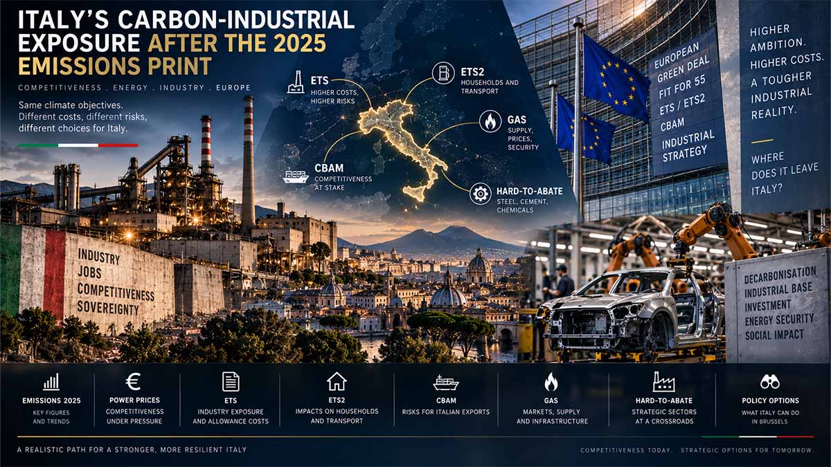
Scope: This dossier examines Italy’s exposure from 2026 through 2030 to the interaction between the EU ETS, ETS2, CBAM, internationally priced gas, electricity-market formation, power-system constraints and the existing Italian hard-to-abate plant stock, with the operative question defined not as whether the European Union should decarbonise but as which instrument should operate on which timetable, with what fiscal, industrial-output and system cost, given Italy’s actual installations, energy infrastructure and import basket.
Executive Summary / BLUF
- Italy’s central exposure is a sequencing problem rather than a dispute over the existence of the EU decarbonisation objective: the domestic system must absorb an accelerating carbon-price architecture at the same time that industrial electrification, storage, renewable generation, hydrogen production and household electrification all compete for grid capacity, while natural gas continues to influence marginal electricity pricing and therefore the cash cost of electricity-intensive industrial substitution.
- The latest official Italian inventory does not yet contain 2025 national inventory emissions: ISPRA’s National Inventory Document 2026 covers 1990–2024, reports 2024 territorial greenhouse-gas emissions excluding LULUCF at just over 363 Mt CO₂eq, approximately 30% below 1990 and 3.6% below 2023, and attributes much of the 2024 decline to increased renewable generation—particularly hydro and wind—energy-efficiency improvement and fuel substitution; consequently, a definitive decomposition of the 2025 Italian decline into policy, weather, hydro and industrial-output components cannot yet be claimed from the Italian UNFCCC inventory. National Inventory Document 2026. Italian Greenhouse Gas Inventory 1990–2024 — ISPRA ISPRA
- The companion EDGAR_2026_GHG account is therefore useful for the 2025 international comparison but must not replace the Italian inventory: EDGAR explicitly reports greenhouse-gas emissions excluding LULUCF and separately publishes fossil CO₂, meaning that GHG and fossil CO₂ are different accounting perimeters and will not be mixed anywhere in this dossier. GHG emissions of all world countries — 2026 Report — JRC/EDGAR edgar.jrc.ec.europa.eu
- The legal timetable has materially changed and is now settled at primary-law level for the purposes of this brief: Regulation (EU) 2026/667, adopted on 11 March 2026, made the Union’s 2040 target a binding 90% reduction in net greenhouse-gas emissions versus 1990, while separately postponing operation of ETS2 for buildings, road transport and additional sectors until 2028. Regulation (EU) 2026/667 — EUR-Lex Eur-Lex
- ETS2 nevertheless becomes a price-formation issue before it becomes a surrender-compliance issue: EEX published the first 2027 ETS2 auction calendar on 30 September 2026, with auctions scheduled from 18 January to 20 December 2027 and an aggregate scheduled 2027 volume of 293,217,500 ETS2 allowances, so Rome’s household, transport and fiscal-incidence analysis must be completed before the market begins discovering a cash price. EEX publishes revised 2027 calendar for EU ETS1 auctions and new 2027 calendar for EU ETS2 auctions — 30 September 2026 EEX
- CBAM is already in its definitive phase, but 2026 should not be described as a mature steady-state carbon border cost: certificate pricing follows the EU ETS auction price, using a quarterly weighted average in 2026 and a weekly average from 2027, while the economic liability must be assessed together with the declining free-allocation adjustment, origin-specific embedded-emissions data and any carbon price demonstrably paid in the country of production. CBAM definitive regime — European Commission Price of CBAM certificates — European Commission Taxation and Customs Union
- The electricity-system constraint is not a shortage of nominal project interest: Terna recorded 328,977 MW of renewable-generation connection requests with accepted STMG status at 31 December 2025, including 139,006 MW in the South, 74,426 MW in Sicily and 47,520 MW in Sardinia, whereas the policy problem is the conversion of those requests into authorised, financed, connected and dispatchable assets, together with the storage and network capability required to convert intermittent capacity into industrially usable energy. Connection requests for new renewable plants — Terna Terna
- Storage procurement has moved from policy design into execution but remains only one component of the closure test: Terna’s first MACSE auction, held on 30 September 2025, awarded 10 GWh of storage capacity for operation from 2028, with a weighted-average clearing price of €12,959/MWh-year; meanwhile, RSE has reconstructed the complete 2030 PNIEC Policy Scenario in IEA energy-balance format, allowing the dossier to test the plan against low-hydro and accelerated-electrification conditions rather than simply repeat installed-capacity objectives. Terna completes first MACSE auction: 10 GWh of energy storage capacity awarded — Terna The energy balance of the Italian NECP to 2030 — RSE Terna Download
- The cabinet decision is therefore not reducible to an ETS price forecast: by the time the dossier reaches its final action chapter, every instrument will be tested against four separate quantities—Italian territorial tonnes, global tonnes after trade substitution, Italian fiscal transfer and Italian industrial gross value added/output—and where the last quantity cannot be calculated from verified establishment-level evidence, the report will state “not in source” rather than substitute a generic multiplier.
Italy’s Carbon Constraint Is Now an Industrial-Timing Problem
Italy’s carbon policy is entering a phase in which the binding question is no longer whether emissions fall, but whether they fall through technological substitution or through lost domestic output. The contradiction is already measurable: territorial greenhouse-gas emissions excluding LULUCF fell to 363.49 MtCO₂eq in 2024, while the official 2030 policy scenario points to 281.0 MtCO₂eq; at the same time, Terna’s 2030 electricity pathway requires demand to rise toward 362 TWh, solar and wind capacity to approach 107 GW, and new storage requirements to reach 71.5 GWh. Italy is therefore trying to remove another large block of carbon precisely when steel, chemicals, heating and transport increasingly need the electricity infrastructure through which that reduction must occur. The next policy error would be to accelerate one clock while assuming that the others will automatically follow.
The 2025 emissions print is not yet a settled policy success
The latest consolidated Italian inventory stops at 2024. ISPRA’s National Inventory Document 2026 records 363.49 MtCO₂eq of greenhouse-gas emissions excluding LULUCF, about 30.2% below 1990, with energy still representing roughly 81% of gross territorial emissions. Inside that total, energy-industry emissions fell strongly and manufacturing-combustion emissions also declined, while transport moved in the opposite direction, adding roughly 4.4 MtCO₂eq in 2024. The accounting result is therefore already economically ambiguous: one tonne disappears because power generation changes, another because an industrial line runs less, while transport can offset both.
The ambiguity becomes larger in 2025. EDGAR’s 2026 emissions account estimates the Italy/San Marino/Holy See aggregate at 354.44 MtCO₂eq, against 362.66 Mt in 2024, implying a decline of about 8.22 Mt. ISPRA’s national 2025 trend estimate, however, pointed to a 0.3% increase, principally because gas consumption for electricity generation rose by approximately 2.5% as hydro weakened, with electricity-sector emissions estimated up 1.2%. These are different methodologies and perimeters, not numbers that can be averaged. Until the consolidated Italian inventory resolves them, 2025 cannot credibly be presented as proof that structural decarbonisation is proceeding exactly as planned.
The carbon burden is moving into harder parts of the economy
Italy’s stationary ETS emissions were approximately 101.4 MtCO₂eq in 2024, including 60.4 Mt from power and heat installations and 41.0 Mt from industrial installations. The reduction since 2013 has been substantially faster in power than in industry, while the remaining non-ETS burden is concentrated in transport, buildings, agriculture and smaller combustion sources. That changes the political economy of the next tonne: ETS2 begins operating in 2028, reaching road fuels and buildings after the original ETS system had concentrated heavily on a comparatively small population of large installations.
Industry is equally heterogeneous. Under Commission Implementing Regulation (EU) 2026/1412, the 2026–2030 free-allocation benchmarks include 1.248 allowances/t of hot metal, 0.142/t for EAF carbon steel, 0.656/t for grey clinker, 1.423/t for aluminium, 1.522/t for ammonia and 0.394/t for float glass. Under current law the CBAM factor remains 97.5% in 2026, falls to 90% in 2028 and reaches 51.5% in 2030. An installation whose technology does not change can therefore face a radically different uncovered carbon position within four years simply because the regulatory protection around that technology changes.
Some plants face a carbon problem; others face a power problem
The distinction is clearest in steel. A BF-BOF route emits roughly 1.9 tCO₂ per tonne of crude steel, giving a gross carbon value of €114/t at €60 per allowance, €161.50/t at €85 and €228/t at €120. The replacement route exists—DRI followed by EAF, potentially using hydrogen—but the JRC route analysed in the dossier requires around 4 MWh of electricity per tonne of steel. One million tonnes of annual production therefore implies approximately 4 TWh of electricity, equivalent to an average continuous load of roughly 457 MW before wider site consumption.
Scrap-EAF steel has almost the opposite exposure. Direct emissions are around 0.06–0.10 tCO₂/t, but electricity demand is roughly 500 kWh/t; a €50/MWh power-price movement therefore shifts production cost by about €25/t before rolling and finishing. Primary aluminium is more extreme: the JRC reference electricity intensity is 14.79 MWh/t, making every €10/MWh movement worth about €148/t aluminium. A generic “industrial carbon” instrument would therefore compensate fundamentally different risks under one label.
Ammonia converts the same problem into network scale. Conventional production emits roughly 1.6–1.9 tCO₂/t NH₃, while an electrolytic route requires around 10–12 MWh/t ammonia. An 800,000 t/y plant supplied through electrolysis therefore needs around 8 TWh/y, corresponding to an average load close to 913 MW. The carbon price can weaken the economics of the fossil route; it cannot create the substation, transmission capacity, renewable generation and hydrogen equipment required by the replacement route.
ETS2 turns carbon pricing into household distribution
The timetable is now precise: ETS2 operates from 2028, but the first auctions start on 18 January 2027, according to the European Commission’s 2027 auction calendar. Using the official fuel factors adopted in the dossier, household natural gas carries an incremental carbon cost of approximately €0.108/Smc at €50/tCO₂, €0.162 at €75 and €0.216 at €100. For the ARERA reference vulnerable household in climatic zone F consuming 1,105 Smc/y, the resulting gross annual cost is about €119, €179 and €239 respectively.
Road fuel adds a second channel. Diesel carries approximately 2.62 kgCO₂/litre under the reference conversion used in the dossier, corresponding to about €0.131/L at €50/t, €0.196/L at €75 and €0.262/L at €100. Combining the zone-F gas reference with 1,000 litres of diesel annually produces a gross carbon incidence of roughly €501/y at €100/tCO₂ before recycling. Italy has submitted its Social Climate Plan, but the Commission still records it as under assessment; the exact approved household allocation is therefore [NOT IN DOSSIER].
The distributional tension is consequently more precise than the language usually surrounding ETS2. A low-income renter in climatic zone F with an inefficient gas-heated dwelling and unavoidable road travel can face materially greater incidence than an urban household with the same income but little heating and no car, while a high-income household may pay more euros but a much smaller share of disposable income. A national average conceals the variable the Social Climate Fund is meant to address.
CBAM becomes much harder after the apparently soft first year
The definitive CBAM regime has applied since 1 January 2026, but 2026 understates its later impact because residual free allocation remains high and the default uplift remains comparatively small. In the dossier’s worked example, a 5,000-tonne Turkish BF-BOF flat-steel cargo produces adjusted embedded emissions of 13,354 tCO₂e in 2026 after the 10% default uplift. Following the free-allocation adjustment, the requirement is about 6,675 certificates; at the official Q2 2026 CBAM certificate price of €75.28/tCO₂, the net cost is roughly €503,000.
By 2030, the same physical cargo faces a 30% default uplift and a current-law CBAM factor of 51.5%. The net certificate requirement rises to about 12,254, approximately 83.6% above the 2026 requirement. At an €85/t sensitivity, the net border cost becomes roughly €1.04 million, or about €208/t steel. The 10,000-tonne Algerian grey-clinker example moves in the same direction, from approximately 7,587 net certificates in 2026 to 13,210 in 2030.
That is why the Commission’s 17 July 2026 ETS revision proposal has immediate industrial significance. Current law takes the CBAM factor to 51.5% in 2030; the proposal would leave it at 59%. The difference is 7.5 percentage points of residual protection, and for a capital-intensive plant deciding whether a replacement process can be commissioned before protection falls, that is a financing variable rather than a semantic adjustment.
The PNIEC works only if its physical assumptions arrive together
Terna’s 2030 policy case is built around approximately 362 TWh of demand, around 107 GW of solar and wind, renewable generation covering roughly 63% of electricity consumption, and a requirement for 71.5 GWh of new storage net of existing pumping. The first MACSE auction awarded 10 GWh for delivery from 2028, while Capacity Market auctions covering 2022–2027 historically secured about 10.5 GW of new firm capacity, of which roughly 1.5 GW was subsequently terminated. The transition is therefore not a renewable target; it is a chain in which generation, storage, firm capacity and transmission must all arrive on schedule.
Hydro exposes the weakness of treating annual capacity as guaranteed energy. In 2022, Italian hydro production fell by 17.2 TWh from the previous year. Applying the same physical shock to the 2030 balance reduces the renewable contribution from about 228 TWh to 211 TWh, taking its implied share from 63% to roughly 58.3% unless another source fills the gap. If electrification simultaneously pushes demand 20 TWh above the PNIEC trajectory, the residual system requirement rises by about 37.2 TWh relative to the central case, equivalent to approximately 4.25 GW of average annual supply before peak coincidence.
Italy can cover such a gap, but every option has a counter-cost. Net imports were 46.9 TWh in 2025, yet the 2022 adequacy episode demonstrated that drought, thermal constraints and weaker import availability can coincide. Gas remains the principal dispatchable backstop; batteries can shift energy only if they were charged beforehand; and demand response becomes an industrial-output question when the adjustable load is an EAF, chemical plant or continuous furnace.
The next 12–24 months will determine whether Italy removes carbon or production
ISPRA’s 2030 WAM scenario reaches 281.0 MtCO₂eq excluding LULUCF, about 82.5 Mt below 2024, while the WM reference case remains at 338.62 Mt, leaving a 57.62 Mt gap between the two policy pathways. That figure cannot be assigned to ETS2, CBAM or ETS1 alone because the WAM contains a broader PNIEC package; its significance is that the official policy path expects a large emissions reduction while still assuming continued physical output in steel, cement, glass and paper.
During the next 12–24 months, the decisive state capacity is therefore informational as much as legislative: Italy needs plant-level ETS1 allowance deficits, 2027–28 electricity hedge coverage, CBAM defaults measured against verified actual emissions, ETS2 incidence by income quintile and climatic zone, and an hourly PNIEC closure model under low hydro and accelerated electrification. Without those records, an Italian tonne can disappear from the inventory without establishing that the tonne disappeared globally, while a poorly designed industrial transfer can preserve current output without financing the technology that removes the liability.
The cost of inaction is identifiable rather than rhetorical. Households pay where ETS2 arrives before structural fuel substitution; electricity-intensive plants pay where grid capacity and procurement contracts lag the carbon timetable; the Treasury pays where compensation is designed after exposure instead of before it; and the industrial base pays where free allocation falls before replacement infrastructure becomes operational. Italy’s choice is therefore not between decarbonisation and non-decarbonisation. It is whether the same 2030 emissions objective is reached through investible technological substitution, or partly through the disappearance of production that the country then buys back from somewhere else.
Navigational Index
Pillar I — The Italian Carbon Account and the Price Transmission Mechanism
Chapter 1 — Decision Sheet
Four decisions only, each attached to a date by which Rome must act, and each expressed through the requested hold / amend / condition architecture: ETS2 national implementation and the Social Climate Plan; CBAM authorised-declarant coverage and challenges to official default values; the 2027–28 industrial power-price hedge; and the Italian negotiating position on the 17 July 2026 ETS review and implementation of the binding 2040 target.
Chapter 2 — Italian Emissions Identity
A reconciled accounting table for 1990, 2005, 2019, 2024 and 2025, separating territorial GHG, ETS1, non-ETS, LULUCF and consumption-based emissions where a robust official series exists, followed by a sector split covering power, industry, transport, buildings, agriculture and waste and an explicit test of whether the observed decline reflects policy abatement, hydro/weather effects, structural fuel substitution or lower industrial output.
Chapter 3 — The Industrial Electricity Price Stack
A bottom-up reconstruction of one industrial kilowatt-hour delivered in the North, Sicily and Sardinia, separating zonal wholesale energy, dispatching, capacity remuneration, MACSE where economically applicable, transmission, distribution, system charges, taxes and the ETS component already embedded through fossil marginal generation, followed by like-for-like comparison with German and French industrial customers on the relevant spot day and on a 2024 annual-average basis.
Pillar II — Plant Economics, Household Incidence and the Carbon Border
Chapter 4 — Plant-Level Exposure, Not Sector Slogans
Installation-route analysis for BF-BOF steel, EAF steel, clinker, primary aluminium, ammonia/fertilisers, refining and float glass, including direct process emissions, free-allocation exposure in 2026, 2028 and 2030, cash-cost sensitivity at €60, €85 and €120/t EUA, import parity after CBAM, and the physical replacement pathway available at engineering level—DRI, EAF/scrap intensification, CCS, fuel switching, electrolytic hydrogen, electrification or closure—together with the associated electricity, hydrogen and network call.
Chapter 5 — ETS2 Incidence on Italian Households and Mobility
A distributional model for household natural gas and road diesel in 2028 and 2030, calculated at three carbon-price levels and presented before and after Social Climate Fund recycling, with results segmented by income quintile and climatic zone and with a separate determination of what the public record actually establishes about building electrification, distribution-grid constraints and connection queues.
Chapter 6 — CBAM Mechanics and the Italian Import Basket
A worked legal-economic calculation for 5,000 tonnes of BF-BOF flat steel and 10,000 tonnes of clinker, using the official Commission default-value methodology, the relevant 2026 CBAM adjustment and the scheduled 2030 free-allocation decline, while separating gross embedded carbon value from net certificate liability and testing the principal circumvention pathways: downstream processing outside present scope, resource shuffling, CN-code manipulation and default-value gaming.
Pillar III — System Closure, 2030 Scenarios and the Twelve-Month State Programme
Chapter 7 — System Constraint and the PNIEC Closure Test
A physical balance of renewable connection requests, storage, hydro flexibility, coal/oil phase-down, residual gas generation, interconnector capability and zonal constraints, followed by two explicit 2030 stress cases—low hydro and accelerated electrification through heat pumps, industrial substitution and ETS2 response—to determine whether the PNIEC balance still closes and, if not, whether the residual adjustment must come from industrial demand, electricity exports/imports, dispatchable fossil output or the timetable of the target itself.
Chapter 8 — Three Scenarios to 2030
Exactly three architectures: Instruments Held, with ETS2 operating from 2028, CBAM/free-allocation adjustment continuing as legislated and EUA sensitivity at €80–100/t; Instruments Conditioned, with ETS2 incidence controls, a CBAM perimeter matched more closely to the actual import basket and an industrial PPA/capacity architecture; and Instruments Slipped, with a further ETS2 delay and a freeze or slowing of the CBAM/free-allocation transition, including the associated Council/legal consequences. Every scenario ends with an Italian tonne delta and Italian gross-value-added delta, or with “not in source” where the latter cannot be calculated defensibly.
Chapter 9 — Twelve-Month Action List
A maximum of eight operational actions, each carrying an institutional owner drawn from MASE, MIMIT, MEF, MAECI, ISPRA, GSE and Terna, a twelve-month deliverable, an identified budget line or an explicit statement that the line is not in the public source, and a falsification condition specifying the evidence that would terminate the proposed action; mandatory deliverables will include a plant-level ETS1 cash-cost register, a CBAM default-value challenge file, an ETS2 incidence model by quintile and climatic zone before the 2027 auctions, and an explicit decision on zonal industrial tariff treatment of Sicily and Sardinia.
Master Abstract
Italy’s position inside the post-2025 European carbon-industrial architecture cannot be evaluated reliably by comparing aggregate national emissions with the European Union’s aggregate trajectory, because the remaining Italian reduction problem is becoming progressively more concentrated in the parts of the economy where carbon-policy instruments intersect most directly with physical capital: transport fleets, gas-heated buildings, high-temperature industrial furnaces, steelmaking routes, clinker kilns, ammonia and hydrogen production, refining, primary metals and electricity-intensive manufacturing. The most recent Italian official inventory confirms that national greenhouse-gas emissions excluding LULUCF were a little above 363 Mt CO₂eq in 2024, approximately 30% below 1990 and 3.6% below 2023, but the same ISPRA record attributes a material part of that year’s reduction to renewable-generation conditions, particularly hydro and wind, together with efficiency and fuel substitution; the official Italian inventory does not yet provide a 2025 sectoral decomposition that would justify treating the following year’s decline as entirely structural. National Inventory Document 2026. Italian Greenhouse Gas Inventory 1990–2024 — ISPRA ISPRA
The companion EDGAR account therefore serves a different function: it gives the dossier a harmonised 2025 international emissions print, but the report will use it only where an Italian tonne changes the global inference and will not substitute EDGAR’s internationally harmonised country estimate for the national UNFCCC inventory. EDGAR explicitly separates total GHG excluding LULUCF from fossil CO₂, and its downloadable files distinguish gases, sectors and countries; this is important because the political meaning of a national GHG decline changes substantially depending on whether the fall comes from power-sector substitution, lower industrial activity, transport demand, methane or another source. GHG emissions of all world countries — 2026 Report — JRC/EDGAR edgar.jrc.ec.europa.eu
The legal environment has meanwhile become more demanding but also more precisely defined. Regulation (EU) 2026/667 amended the European Climate Law by establishing a binding 2040 net-GHG reduction target of 90% against 1990, while allowing the post-2030 implementation architecture to consider elements including international credits, permanent removals, cross-sector flexibility, investment needs and industrial competitiveness; the same instrument separately postpones ETS2 operation until 2028. Regulation (EU) 2026/667 — EUR-Lex Eur-Lex This matters for Italy because the operative negotiating question in Brussels is no longer whether a 2040 target will exist, but how the legislation implementing that binding target will distribute the burden among ETS1 installations, ETS2 sectors, removals, electricity consumers and imported carbon-intensive goods.
ETS2 illustrates the distinction between a legal compliance date and an economic preparation date. Its operation is postponed until 2028, but EEX has already published the 2027 auction calendar, with the first auction scheduled for 18 January 2027 and an overall 2027 volume of 293.2175 million ETS2 allowances. EEX publishes revised 2027 calendar for EU ETS1 auctions and new 2027 calendar for EU ETS2 auctions — 30 September 2026 EEX For Rome, that creates a hard administrative deadline: the incidence of the new carbon price on household heating and road transport must be quantified by income, climatic geography and fuel use before the market begins to establish a reference price, because compensation designed after price formation will have weaker targeting and a larger risk of becoming an indiscriminate fiscal transfer.
CBAM has the opposite problem: the definitive regime is already legally operational, but 2026 is not economically representative of its later steady-state burden. The Commission states that the price of CBAM certificates is linked to EU ETS auction prices, calculated quarterly in 2026 and weekly from 2027, while carbon prices demonstrably paid in the country of origin can reduce the obligation. CBAM definitive regime — European Commission Price of CBAM certificates — European Commission Taxation and Customs Union The cabinet consequence is that there is no analytically valid single number called “the CBAM cost”: a steel cargo, clinker cargo or fertiliser shipment must be evaluated by product code, origin, production route, embedded emissions, official default or verified actual value, carbon price already paid and the corresponding free-allocation adjustment for the year being modelled.
The industrial problem is consequently plant-specific. An Italian BF-BOF steel installation faces a different direct-carbon path from an EAF mill; a clinker kiln combines process calcination with fuel combustion; primary aluminium is dominated by electricity economics; ammonia is simultaneously exposed to gas feedstock, hydrogen chemistry and future electrolyser power demand; refineries require high-temperature process heat and hydrogen; and float glass cannot convert simply because wholesale renewable capacity exists somewhere in the national system. The relevant question for each installation is whether the compliant replacement route exists at engineering level, whether the infrastructure required by that route can reach the plant, and whether the replacement route can operate at a power or hydrogen cost that preserves a viable margin before the legacy route loses free allocation or incurs higher allowance expense.
That dependence shifts the analysis directly into electricity-system physics. Terna reported 328.977 GW of renewable connection requests with accepted STMG status at the end of 2025, distributed heavily toward the South, Sicily and Sardinia. Connection requests for new renewable plants — Terna Terna The figure is strategically important precisely because it demonstrates that Italy does not lack nominal investor interest in renewable capacity; the constraint lies in converting that pipeline into permitted and financed generation, reinforcing transmission corridors, procuring enough storage and firm capacity, and ensuring that the resulting electricity is deliverable at the location and hour required by an industrial installation. The first MACSE auction has already moved 10 GWh of storage into contracted delivery for 2028, while RSE’s reconstruction of the 2030 PNIEC Policy Scenario provides a sufficiently structured energy balance to test whether the plan remains internally coherent when hydro availability is weak or electrification runs ahead of the central case. Terna completes first MACSE auction: 10 GWh of energy storage capacity awarded — Terna The energy balance of the Italian NECP to 2030 — RSE Terna Download
The resulting Italian negotiating position cannot therefore be built around the proposition that carbon prices are intrinsically either desirable or undesirable. Fact: the Union has legislated a 90% net reduction objective for 2040, ETS2 now starts in 2028, CBAM is in its definitive phase, the ETS review was launched by the Commission on 17 July 2026, and the Italian power system is simultaneously processing a renewable-connection pipeline whose nominal capacity far exceeds foreseeable incremental demand. EU Emissions Trading System — European Commission, 17 July 2026 revision notice Climate Action Inference: the binding constraint increasingly becomes the synchronisation of carbon-cost exposure with the physical availability of lower-carbon replacement routes. Judgement for testing in this dossier: an instrument that removes an Italian tonne by replacing technology has a different strategic value from an instrument that removes the same territorial tonne by lowering Italian industrial output and replacing it with imported production; therefore every chapter must distinguish the carbon account from the production account rather than use emissions alone as the measure of policy effectiveness.
Key Evidence Table
| Indicator | Value / status | Reference date | Definition / scope | Issuer | Exact source |
|---|---|---|---|---|---|
| Italian territorial GHG emissions excluding LULUCF | Just over 363 Mt CO₂eq; −3.6% y/y; approximately −30% versus 1990 | 2024 | Official Italian national GHG inventory, excluding LULUCF | ISPRA / Italian UNFCCC submission | National Inventory Document 2026. Italian Greenhouse Gas Inventory 1990–2024 ISPRA |
| Italian official inventory coverage | 1990–2024 | Submitted 10 Apr 2026 | National Inventory Document under UNFCCC/Paris Agreement reporting | Italy / UNFCCC | Italy. 2026 National Inventory Document (NID) UNFCCC |
| EDGAR 2026 perimeter | GHG excluding LULUCF; fossil CO₂ separately reported | 2025 data vintage in 2026 report | Internationally harmonised emissions account, not interchangeable with Italian NID | JRC / IEA-EDGAR | GHG emissions of all world countries — 2026 Report edgar.jrc.ec.europa.eu |
| EU 2040 target | −90% net GHG versus 1990, binding | Regulation adopted 11 Mar 2026 | Union-wide net GHG target after removals | European Parliament / Council | Regulation (EU) 2026/667 Eur-Lex |
| ETS2 operation | Postponed until 2028 | Regulation adopted 11 Mar 2026 | Buildings, road transport and additional sectors under Chapter IVa ETS Directive | European Parliament / Council | Regulation (EU) 2026/667, Article 2 Eur-Lex |
| First ETS2 auction | 18 Jan 2027 | Calendar published 30 Sep 2026 | Common auction platform | EEX / Commission / Member States | EEX 2027 ETS2 Auction Calendar announcement EEX |
| 2027 ETS2 auction volume | 293,217,500 ETS2A | 2027 | Scheduled common-platform allowance volume, including SCF-related allowances | EEX | EEX 2027 ETS2 Auction Calendar announcement EEX |
| CBAM regime | Definitive phase operational | From 1 Jan 2026 | Cement, iron and steel, aluminium, fertilisers, electricity and hydrogen under the CBAM Regulation | European Commission | CBAM definitive regime Taxation and Customs Union |
| CBAM certificate pricing | Quarterly EU ETS auction-price average in 2026; weekly from 2027 | 2026– | Weighted auction-price methodology | European Commission | Price of CBAM certificates Taxation and Customs Union |
| Renewable connection queue | 328,977 MW; 5,921 accepted-STMG procedures | 31 Dec 2025 | New renewable-generation connection requests | Terna | Connection requests for new renewable plants Terna |
| Sicily renewable requests | 74,426 MW | 31 Dec 2025 | Accepted STMG renewable requests | Terna | Connection requests for new renewable plants Terna |
| Sardinia renewable requests | 47,520 MW | 31 Dec 2025 | Accepted STMG renewable requests | Terna | Connection requests for new renewable plants Terna |
| First MACSE auction | 10 GWh contracted; €12,959/MWh-year weighted-average clearing price | Auction 30 Sep 2025; delivery from 2028 | Electricity-storage procurement in Central-South, South/Calabria, Sicily and Sardinia | Terna | Terna completes first MACSE auction: 10 GWh of energy storage capacity awarded Terna Download |
| PNIEC 2030 energy balance | Full Policy Scenario reconstructed in IEA-format balance | 2030 scenario | National energy-system balance consistent with PNIEC 2024 | RSE | The energy balance of the Italian NECP to 2030 RSE Web |
| ETS legislative review | Commission targeted revision proposed | 17 Jul 2026 | EU ETS post-2030/industrial-competitiveness revision package | European Commission | EU Emissions Trading System — Commission Climate Action |
Analytical Pathways
A formal Analysis of Competing Hypotheses is not activated at this stage, because the decision problem is not a question of choosing among three mutually exclusive hidden intentions or explanations and the evidentiary prerequisites specified by the governing protocol are therefore not satisfied. The more appropriate architecture is to test three observable pathways throughout the dossier.
Technology-substitution pathway. Italian territorial emissions fall because the underlying production process changes—renewable electricity displaces fossil generation, EAF replaces or supplements BF-BOF steelmaking, hydrogen or CCS changes ammonia and refining emissions, industrial furnaces change fuel, buildings electrify, or transport shifts propulsion technology. This pathway produces a genuine reduction in domestic process carbon without requiring equivalent contraction of physical output, although its global effectiveness still depends on upstream power, imported hydrogen, materials and supply-chain effects.
Output-contraction pathway. Italian territorial emissions fall because industrial utilisation, transport activity or energy demand contracts rather than because the production technology has been replaced. In this case an emissions target can be achieved statistically while industrial value added, employment or strategic production capacity deteriorates, and part of the apparent carbon benefit can be reversed globally if higher-emission imports replace the lost Italian output.
Mixed substitution-leakage pathway. Domestic plants reduce emissions and output simultaneously while CBAM, free allocation, electricity prices and import competition redistribute production among EU and non-EU facilities. This is the most analytically demanding pathway because the Italian territorial carbon account, the European industrial account and the global atmospheric account can move in different directions; the chapter sequence is therefore designed to calculate those three effects separately rather than infer one from another.
Principal Gaps and Watch Indicators
Italian 2025 inventory decomposition. EDGAR supplies an international 2025 estimate, but the latest Italian UNFCCC inventory stops at 2024; therefore the precise division of the 2025 Italian change among power generation, industrial output, transport, buildings, agriculture and waste remains an official-record gap that can change the attribution of the entire 2025 print. Italy. 2026 National Inventory Document — UNFCCC UNFCCC
Plant-level ETS cash exposure. Installation emissions and allocations can be assembled from registry and national-authority records, but a government-ready dataset linking verified emissions, actual output, production route, free allocation, procurement price, conversion capex and closure risk is not published as one integrated Italian instrument; that missing bridge is critical because sector averages cannot distinguish BF-BOF from EAF economics or an electricity-intensive plant already hedged through long-term contracts from one purchasing against short-term market prices.
Final Italian Social Climate Plan financing and incidence map. The dossier will separate the statutory EU funding architecture from the value actually available under Italy’s final accepted national plan; no euro figure will be attributed to the Italian plan until it has been extracted from the relevant Commission/Italian official instrument rather than inferred from Italy’s theoretical share of the EU envelope.
2027 ETS2 price formation. The first hard signpost is now fixed: 18 January 2027. The first weeks of ETS2 auctions will reveal whether the market clears near policy-model assumptions or at a materially higher level and will therefore determine the first empirical household and road-fuel incidence range. EU ETS2 Auctions — EEX EEX
CBAM default values and Italian origin mix. The legally correct cash exposure of Italian importers depends on exact CN code, country of origin, production route, actual or default embedded-emissions value, carbon price already paid and the free-allocation adjustment; operator counts or generic average embedded-emission factors will therefore remain provisional until reconciled with the Commission tables and ISPRA’s role as the Italian competent authority.
Power-price normalisation versus structural premium. The 3 October 2026 spot print identified in the user’s anchor set is a market observation, not a forward planning price; Chapter 3 will therefore distinguish the spot day from the 2024 annual industrial-price comparison and from the range required for a 2027–28 hedge decision, because using the current stressed day-ahead print as the planning value would contaminate every plant-level calculation.
Network conversion of the renewable queue. Terna’s 328.977 GW accepted-STMG pipeline measures connection requests, not commissioned renewable capacity, and therefore the relevant watch indicators are authorisation, construction, grid reinforcement, storage commissioning, curtailment, zonal congestion and the commissioning profile of projects in the South and the islands rather than the nominal size of the queue itself. Connection requests for new renewable plants — Terna Terna
MACSE delivery performance. The first 10 GWh of contracted storage enters operation from 2028, making project commissioning and technology performance an observable test of whether storage procurement is arriving quickly enough to support the PNIEC and industrial-electrification trajectories. Terna completes first MACSE auction: 10 GWh of energy storage capacity awarded Terna Download
Post-2030 ETS legislation. The Commission’s 17 July 2026 targeted revision opens the principal legal window in which Italy can seek changes to the interaction of competitiveness, free allocation, benchmarks, industrial support and the 2040 trajectory; the decisive watch indicators are therefore the Council working-party text, Parliament amendments, Commission impact-assessment assumptions and any changes to the legal treatment of industrial removals, free allocation or CBAM-covered production. EU Emissions Trading System — European Commission Climate Action
Decision Logic Governing the Chapters
The dossier will maintain three analytical separations from the first decision sheet to the final action list.
Fact will be stated independently of inference. For example, it is a fact that ETS2 has been postponed to 2028 and that the 2027 auction calendar now exists. Regulation (EU) 2026/667 EEX 2027 ETS2 Auction Calendar announcement Eur-Lex It is an inference that January 2027 price discovery makes the household-incidence model an urgent 2026 administrative task. It will be a cabinet judgement, not an analytical fact, whether that evidence supports holding, amending or conditioning the instrument.
Territorial carbon will be separated from global carbon. A tonne disappearing from the Italian inventory because a plant changes technology is not economically or atmospherically equivalent to a tonne disappearing because the same production relocates to a foreign installation with a different carbon intensity. EDGAR will therefore be invoked only at the point where an Italian change must be translated into the global account, exactly as required in the task specification. GHG emissions of all world countries — 2026 Report — JRC/EDGAR edgar.jrc.ec.europa.eu
Carbon cost will be separated from energy-system cost. An EUA cost is not synonymous with the wholesale electricity price, and the ETS component passed through by a marginal fossil generator cannot simply be added a second time to PUN; similarly, MACSE remuneration, capacity-market payments, transmission investment, distribution charges, taxes and gas commodity costs must remain separate layers so ministers can identify which cost is governed in Rome, which is generated by a European instrument and which is driven by internationally traded fuel.
Italy’s Carbon-Industrial Exposure After the 2025 Emissions Print
Decision architecture for the Presidency of the Council of Ministers on the interaction between EU ETS1, ETS2, CBAM, gas-linked power pricing, industrial competitiveness, electricity-system adequacy and the physical decarbonisation capacity of Italy’s hard-to-abate plant base through 2030.
Command and Analytical Roles
Institutional responsibility is separated from evidence production and political decision.Lead Principal Intelligence Analyst and Multi-Domain Synthesis Architect
Acts as lead drafter for the Presidency of the Council of Ministers and integrates legal, energy, industrial, fiscal, trade and infrastructure evidence into a single decision-grade cabinet assessment. The analytical role establishes the strongest defensible public-record account but does not substitute analytical judgement for ministerial political authority.
Strategic coordination, inter-ministerial arbitration and final cabinet decision.
ETS architecture, PNIEC, energy system, climate implementation and EU energy negotiations.
Industrial exposure, hard-to-abate plants, industrial electricity and competitiveness effects.
Fiscal incidence, ETS2 redistribution, taxation, auction revenue and state-aid implications.
Council positioning, coalition building and diplomatic cost of hold, amend or condition strategies.
Evidence production: emissions, CBAM authority, grid adequacy, connection queues and energy-system implementation.
Cabinet Decision Chain
Every policy proposition must move through the same evidentiary sequence.The Four Decisions Rome Must Take
No fifth strategic theme enters the Chapter 1 decision sheet.ETS2 Implementation and Social Climate Plan
Critical window: before 18 January 2027Establish household and transport incidence before ETS2 auctions create a market reference price and before 2028 compliance begins.
CBAM Declarant Coverage and Default-Value Challenge
Critical window: Q4 2026–Q1 2027Match CN code, origin, production route, embedded emissions and operator evidence before default assumptions harden into compliance practice.
2027–28 Industrial Power-Price Hedge
Critical window: before 2027 procurement books closeSeparate gas and ETS exposure from grid, tariff and contractual components before defining any PPA, hedge or targeted industrial mechanism.
ETS Review and 2040 Implementation Position
Critical window: Council negotiations through 2027Determine Italy’s position on the July 2026 ETS revision and the implementation architecture required by the binding 2040 −90% net-GHG target.
Three-Pillar Dossier Architecture
Nine chapters convert the decision problem into auditable evidence.Pillar I — Carbon Account and Price Transmission
Establish what Italy emits, where the emissions occur and how European carbon and energy prices become Italian cash costs.
Pillar II — Plant Economics and Household Incidence
Translate abstract regulatory instruments into physical installations, household budgets and real import transactions.
Pillar III — System Closure and State Action
Test whether the power system can physically support the regulatory trajectory and convert the result into an executable twelve-month programme.
Evidence and Judgement Discipline
Claims are not allowed to move directly from source to political recommendation.FACT
Directly established by legislation, regulator data, official statistics, market data, registry information or another competent first-order source.
INFERENCE
Analytical consequence derived transparently from verified inputs, with the causal mechanism and relevant countervailing forces stated.
JUDGEMENT
Decision-relevant assessment that remains distinct from fact and ultimately requires ministerial choice among available policy positions.
Accounting Separations That Cannot Be Collapsed
These distinctions govern all quantitative chapters.| Variable A | Must remain separate from | Reason | Cabinet relevance |
|---|---|---|---|
| Italian territorial GHG | Global GHG | A domestic reduction can reflect technology substitution, lower output or relocation. | Prevents territorial accounting from being mistaken for global climate effect. |
| Total GHG | Fossil CO₂ | Different gases and accounting perimeters produce different totals and policy implications. | Prevents false comparison between EDGAR series and national inventory categories. |
| EUA cost | Wholesale electricity price | ETS pass-through can already be embedded in marginal fossil-generation bids. | Prevents double-counting carbon in industrial electricity costs. |
| Renewable connection requests | Commissioned generation | Requested MW are not authorised, financed, connected or dispatchable MW. | Prevents nominal project pipelines from being treated as available power supply. |
| CBAM gross embedded cost | Net certificate liability | Free-allocation adjustment and recognised foreign carbon prices modify the obligation. | Prevents a single misleading “CBAM cost” from entering cabinet discussion. |
| Industrial emissions reduction | Industrial decarbonisation | Output contraction can lower emissions without replacing the production technology. | Separates technological transition from deindustrialisation. |
Final Decision Metrics
Every scenario must terminate in measurable consequences.Change in territorial emissions by sector and instrument, with the mechanism responsible for the change identified.
Adjustment for relocation and import substitution where an Italian tonne changes the global emissions inference.
Auction revenue, Social Climate Fund recycling, compensation, taxation effects and public-support exposure.
Industrial production and gross-value-added effect; where the official evidence cannot support the calculation, the dossier prints “not in source”.
Primary Evidence Hierarchy
Lower-tier narrative sources do not replace the controlling record.Pillar I — The Italian Carbon Account and the Price Transmission Mechanism
Chapter 1 — Decision Sheet
Principal judgement
The first twelve months of the Italian carbon-industrial file are governed by four decisions and four clocks, but those clocks do not run at the same speed: ETS2 creates a market-price signal from January 2027 although surrender compliance starts only in 2028; CBAM is already legally operative but its economic bite remains limited by high residual free allocation in 2026; industrial power procurement for 2027–28 is being fixed before the present gas-and-power stress can be known to be temporary or structural; and the Commission’s 17 July 2026 ETS revision has opened a negotiating window in which the post-2030 architecture, industrial free allocation and CBAM interaction can still change before the legally binding 2040 trajectory is translated into the next compliance framework. The appropriate cabinet discipline is therefore not to collapse these files into a generic request for “flexibility”, but to determine separately what Italy would hold, what it would seek to amend, and what it would accept only subject to a defined condition, with each position attached to a quantitative test capable of invalidating it. Climate Action
European Commission — Revised 2027 EU ETS1 and initial 2027 EU ETS2 auction calendars, 1 October 2026
European Commission — EU ETS free-allocation framework and 17 July 2026 revision
Cabinet decision matrix
| Cabinet file | Date by which Rome must have an operative position | HOLD | AMEND | CONDITION | Evidence required before decision |
|---|---|---|---|---|---|
| ETS2 implementation and Social Climate Plan | 18 January 2027, before the first ETS2 auction establishes a market reference price | Implement the 2028 compliance start and existing SCF architecture without seeking alteration to the Union timetable | Seek changes to incidence-management, recycling, auction-supply or national implementation provisions while leaving the 2028 legal start intact | Accept operation from 2028 subject to a predetermined incidence framework linking carbon-price bands to targeted compensation and investment measures | Household gas and road-fuel incidence by quintile, climatic zone and mobility dependence; final Commission assessment of Italy’s Social Climate Plan; national co-financing burden |
| CBAM authorised-declarant coverage and default-value challenge | 31 December 2026 as a cabinet operational deadline, before the first full definitive-regime year closes and ahead of 2027 weekly certificate pricing | Enforce the current 50-tonne threshold, authorisation rules and Commission default methodology as adopted | Seek changes where the Italian CN-code/origin basket shows systematic mismatch between Commission default values and verified production-route emissions | Accept defaults only where Italy cannot demonstrate a statistically material and verifiable divergence using operator evidence | Authorised-declarant universe; imports by CN code/origin; actual versus default embedded emissions; carbon price paid abroad; default-value error distribution |
| 2027–28 industrial power-price hedge | 30 November 2026 as an internal budget/procurement deadline, allowing measures to become operable before 2027 contracting books are substantially fixed | Leave procurement risk with industrial buyers under existing market, PPA and hedging arrangements | Modify available PPA, guarantee, tariff or state-aid architecture for qualifying installations | Make any public instrument contingent upon electricity intensity, plant-level output exposure, hedge coverage, investment obligations and an auditable closure counterfactual | Plant-level load profile; contract/hedge book; voltage level; energy intensity; margin sensitivity; projected output loss at defined €/MWh thresholds |
| 17 July 2026 ETS review and implementation of the 2040 target | 31 March 2027 as an internal negotiating-position deadline, or earlier if the Council working text requires it | Defend the Commission proposal without seeking substantive industrial amendments | Seek changes to post-2030 cap architecture, benchmarks, CBAM/free-allocation interaction, funding or flexibility provisions | Support specified components only where the implementing framework demonstrates an investible replacement route for exposed production rather than relying on output contraction | Italian installation-level ETS exposure, post-2030 benchmark effects, proposed CBAM-factor trajectory, electricity-system closure test and measured GVA exposure |
The dates of 31 December 2026, 30 November 2026 and 31 March 2027 in this table are cabinet planning deadlines, not EU statutory deadlines; they are used because a decision taken after the relevant import year, procurement cycle or negotiating phase would preserve formal legal competence while reducing practical leverage. By contrast, 18 January 2027 is an external market date: the Commission confirmed on 1 October 2026 that ETS2 auctions will start on that date, following publication by EEX on 30 September, even though ETS2 operations themselves begin in 2028. The initial 2027 calendar contains 140 million ETS2 allowances allocated to the Social Climate Fund plus volumes attributable to Member States that had implemented the surrender obligation and excess-emissions penalties when the auction volume was determined, and the Commission has already stated that the auction volumes will be adjusted as additional Member States complete implementation. Climate Action
European Commission — ETS2 auctions begin in January 2027 while operations begin in 2028
Decision One — ETS2 national implementation and the Social Climate Plan
The first decision must be framed around a legal fact that materially changes the sequencing of Italian preparation: ETS2 monitoring and reporting began before compliance, auctioning begins before compliance, and the carbon market will therefore generate price information before regulated entities have to surrender allowances. The Commission had already announced in July that the 2027 ETS2 auction calendar would be published by the end of September; it was then published on 30 September, with the first auction scheduled for 18 January 2027. This eliminates the earlier uncertainty over whether an auction calendar would exist before the end of September 2026 and turns the next Italian decision into a question of incidence management rather than calendar uncertainty. Climate Action
The Social Climate Plan cannot be treated as if its financing were already unconditionally available. The Commission’s current country-status page records Italy as having submitted its Social Climate Plan, with the plan still in the Commission assessment phase, rather than as an adopted plan. This matters because the Presidency’s official implementation tracker separately records the ministerial measure assigning Italian Social Climate Plan resources after EU approval as “not adopted”. The relevant distinction is therefore between the legally maximum national envelope, the plan requested by Italy, the amount eventually approved by the Commission, and the expenditure actually allocated domestically; these figures must not be merged. Employment, Social Affairs and Inclusion
European Commission — Social Climate Fund national plans: Italy submitted, Commission assessment phase
Presidency of the Council — implementation measure for Italian Social Climate Plan resources currently not adopted
The allocation table in the Social Climate Fund Regulation gives Italy a 10.81% distribution share and shows two different monetary ceilings: €7.023970924 billion under the €65 billion architecture and €5.900135577 billion under the lower envelope applicable where ETS2 is postponed to 2028. The ETS Directive itself states that where ETS2 is postponed pursuant to Article 30k, the maximum Social Climate Fund amount falls to €54.6 billion. Those are statutory maximum allocations, not evidence that the final Italian plan has already been approved for €5.900 billion; because the Commission still lists Italy’s plan as under assessment, the plan-specific approved amount is not yet an established final allocation in the opened official record as of 3 October 2026. Eur-Lex
EUR-Lex — Social Climate Fund allocation table, including Italy
The operational meaning of the three postures is therefore narrower than political language normally suggests. A hold posture preserves the 2028 timetable and uses the approved national plan, once approved, as the principal distributional mechanism. An amend posture seeks changes in the way the burden is recycled or in EU-level stabilisation mechanics without reopening the existence of ETS2. A condition posture establishes ex ante national incidence thresholds—expressed, for example, as annual euro cost relative to disposable household income or transport expenditure—and ties the scale and targeting of compensation to those thresholds. None of those alternatives can be assessed from a national average household because heating demand is highly climatic-zone dependent and road-fuel exposure differs sharply between metropolitan households and transport-dependent peripheral households; Chapter 5 will perform that calculation rather than prejudge it here.
Decision Two — CBAM authorised-declarant coverage and default-value challenge
CBAM is no longer a transitional reporting exercise. The definitive regime has applied since 1 January 2026, and importers or indirect customs representatives exceeding the single mass-based 50-tonne threshold for the relevant mass-based sectors must obtain authorised-CBAM-declarant status before importing covered goods, while the first annual CBAM declaration for calendar year 2026 is due by 30 September 2027. The economic price signal is also changing in frequency: the Commission calculates CBAM certificate prices as the weighted average of EU ETS auction clearing prices, quarterly in 2026 and weekly from 2027. For Q1 2026 the published certificate price was €75.36/tCO₂, and for Q2 it was €75.28/tCO₂; the Q3 2026 value is scheduled for publication on 5 October 2026, two days after the date of this brief, and therefore cannot legitimately be inserted here before publication. Taxation and Customs Union
European Commission — CBAM definitive regime and 50-tonne threshold
European Commission — official CBAM certificate prices and methodology
EUR-Lex — consolidated CBAM Regulation, authorised-declarant and declaration rules
A more consequential issue for Rome is that the current law and the Commission’s 17 July 2026 proposal no longer contain the same post-2027 CBAM-factor trajectory. Under current legislation, the factor preserving free allocation for CBAM goods is 97.5% in 2026, 95% in 2027, 90% in 2028, 77.5% in 2029 and 51.5% in 2030, before falling further toward zero. The Commission’s July 2026 proposal would slow that phase-out, with proposed values of 91.5% in 2028, 81% in 2029 and 59% in 2030, and would extend the phase-out beyond the current timetable. This difference is not a technical footnote: for an EU producer whose benchmark entitlement is otherwise unchanged, the proposed 2030 factor would preserve 7.5 percentage points more CBAM-linked free allocation than current law, materially changing the domestic-versus-import parity calculation that Chapter 4 and Chapter 6 will test at plant and cargo level. Eur-Lex
EUR-Lex — current EU ETS Directive CBAM-factor schedule
EUR-Lex — Commission proposal COM(2026) 616 changing the future CBAM-factor trajectory
| CBAM/free-allocation year | Current-law factor | Commission 17 July 2026 proposal | Difference if proposal enacted |
|---|---|---|---|
| 2026 | 97.5% | 97.5% | 0.0 pp |
| 2027 | 95.0% | 95.0% | 0.0 pp |
| 2028 | 90.0% | 91.5% | +1.5 pp |
| 2029 | 77.5% | 81.0% | +3.5 pp |
| 2030 | 51.5% | 59.0% | +7.5 pp |
The hold position in this file means enforcing the authorised-declarant regime, the current threshold and the official default system without seeking a national evidence challenge. The amend position means using verified Italian importer and foreign-plant data to contest a default where the default systematically misstates the production route actually supplying Italy, or supporting EU-level changes to scope where the Italian import basket shows material leakage into downstream products. The condition position means accepting Commission defaults as the administrative fallback but treating verified actual emissions as the preferred basis where the evidence meets legal verification standards. None of these alternatives justifies manipulating a default simply because it increases import cost; a challenge file must demonstrate that the default is technically inaccurate for the relevant origin-product-production-route combination.
Decision Three — the 2027–28 industrial power-price hedge
The third decision is not whether wholesale electricity is “too expensive”, but which component of the delivered industrial price is capable of being addressed through a national instrument without disguising fuel or EU carbon exposure as a domestic network charge. Italy’s 3 October 2026 day-ahead market provides a stress observation rather than an investment planning number: the national PUN Index GME was approximately €181/MWh, while the North, Sicily and Sardinia showed different zonal outcomes; Germany and France cleared below Italy on the same day, but those are wholesale day-ahead comparisons, not comparable delivered industrial bills. A subsidy or hedge based on the whole spot-price difference would therefore risk compensating components that are neither structural nor nationally controllable.
The appropriate industrial file must instead identify four quantities for each materially exposed installation: its unhedged electricity volume, the proportion of its final price generated by market energy rather than regulated/fiscal layers, the output and EBITDA sensitivity to incremental €/MWh, and the maturity date of existing hedges or PPAs. A plant already hedged below a cabinet reference price does not present the same 2027 fiscal exposure as an identical process purchasing substantial volumes against short-term indices, while a plant connected at transmission level does not face the same network tariff architecture as an intermediate industrial customer connected to distribution.
The hold posture leaves that procurement risk with companies under existing contractual structures. The amend posture modifies an existing PPA, guarantee, capacity, tariff or state-aid vehicle for defined classes of installations. The condition posture links access to any public instrument to verified plant-level conditions such as electricity intensity, uncovered purchase volume, production retention, an executable transition investment and an explicit counterfactual showing that the absence of the instrument would create measurable output loss rather than simply lower shareholder return. Chapter 3 establishes the price stack needed to distinguish those effects.
Decision Four — the July 2026 ETS review and the binding 2040 architecture
The fourth decision is the only one that directly changes the architecture beyond the current decade. On 17 July 2026, the Commission proposed a targeted revision of the EU ETS that explicitly addresses industrial competitiveness, free allocation, CBAM interaction, industrial decarbonisation funding, aviation, maritime transport and the gradual extension of emissions trading to municipal-waste incineration. The revision is therefore not an abstract debate about the 2040 target; it is the legislative process through which the carbon-price architecture, protection against leakage and financing of replacement technology are being recalibrated. Climate Action
European Commission — EU Emissions Trading System, 17 July 2026 targeted revision
For Italy the factual baseline is that the ETS cap is already designed to reduce covered emissions 62% by 2030 versus 2005, with the linear reduction factor raised to 4.3% annually for 2024–27 and 4.4% from 2028, together with one-off rebasing reductions of 90 million allowances in 2024 and 27 million in 2026. Any Italian negotiating proposition therefore has to specify what variable it seeks to change—benchmark, phase-out path, funding, scope, flexibility or timing—rather than invoke competitiveness generically. Climate Action
European Commission — EU ETS emissions cap and 2030 trajectory
Chapter 1 decision thresholds
| File | Quantitative evidence that supports preserving the current architecture | Quantitative evidence that strengthens the case for seeking a change | Evidence that makes a national intervention unnecessary |
|---|---|---|---|
| ETS2 | Household incidence remains within pre-defined fiscal/income bands and SCF targeting reaches exposed groups | Actual auction prices and consumption data generate materially higher incidence than the national plan assumed | Market price below planning range combined with negligible incidence after recycling |
| CBAM | Verified actual emissions broadly match official defaults and covered import basket corresponds to material leakage risk | Systematic default error, downstream substitution or uncovered import shift appears in customs data | Differences are statistically and economically immaterial |
| Industrial power | Hedged delivered price remains compatible with plant cash margin and EU peers | Unhedged price differential creates demonstrable production/closure risk not explained by efficiency | Plants already hedged/PPA-covered or price effect too small to alter output |
| ETS review | Current/proposed benchmark and CBAM phase-out leave investible transition route before protection declines | Free allocation declines faster than infrastructure/technology can become operational for documented installations | Replacement projects remain financeable and system capacity is demonstrably available |
The governing principle for the next chapters is therefore empirical rather than rhetorical: a national position must be attached to the variable that produces the cost, because otherwise Rome risks trying to solve an international gas-price shock with a network subsidy, an inadequate network with an ETS amendment, or a genuine carbon-leakage problem with a general industrial transfer.
Chapter 2 — Italian Emissions Identity
The accounting problem comes before the policy interpretation
Italy does not have one single emissions number. The national UNFCCC inventory, the EU ETS registry, the Effort Sharing accounting framework, the LULUCF account and EDGAR each answer different questions, and combining them without perimeter reconciliation produces false arithmetic. The official ISPRA 2026 inventory reports historical national emissions through 2024, whereas EDGAR provides a harmonised estimate for 2025; the EU ETS began only in 2005; ESR/non-ETS accounting excludes a defined set of ETS and aviation emissions rather than simply equalling “territorial total minus industry”; and LULUCF is a signed land-sector net source/sink that must not be buried inside gross territorial emissions. ISPRA
ISPRA — Greenhouse-gas emissions in Italy, reduction targets and scenarios, 2026 edition
ISPRA — Greenhouse Gas Emissions in the ETS and ESR Sectors, updated 30 June 2026
Reconciled emissions identity
All values below are MtCO₂eq unless otherwise stated. Where a series does not exist for the requested year or the opened official record does not provide a comparable number, the cell is explicitly marked rather than synthetically backfilled.
| Accounting perimeter | 1990 | 2005 | 2019 | 2024 | 2025 | Status and interpretation |
|---|---|---|---|---|---|---|
| Territorial GHG excluding LULUCF — Italian national inventory | 520.626 | 593.769 | 411.749 | 363.490 | not in national inventory | UNFCCC/IPCC inventory perimeter; latest consolidated year 2024 |
| ETS1 stationary emissions | N/A — ETS did not exist | ≈225.99 | ≈141.2 | 101.4 | country total not reproduced in the opened official table | EU ETS/Union Registry scope changes over time; values are not directly additive to all national-inventory categories |
| ESD/ESR / non-ETS | N/A | 348.0 regulatory baseline | official series exists; exact cell not reproduced in opened page | approximately 259.7, inferred from ISPRA’s stated 9.6 Mt exceedance against 2024 annual allocation and its published accounting table | latest consolidated national accounting not available as 2025 inventory | Legal compliance perimeter, not simply “everything outside industry” |
| LULUCF net balance | −12.949 | −44.057 | −51.078 | −64.068 in NID table | not in consolidated 2025 inventory | Negative value denotes net removal/sink |
| Territorial GHG including LULUCF | 507.677 | 549.712 | 360.671 | 299.422 | not in consolidated 2025 inventory | Calculated within the same NID table from inventory categories |
| EDGAR GHG excluding LULUCF | separate EDGAR series | separate EDGAR series | separate EDGAR series | 362.66 | 354.44 | Italy + San Marino + Holy See EDGAR aggregate; harmonised estimate, not national inventory |
| Consumption-based GHG footprint | no common official five-year series used | no common official five-year series used | no common official five-year series used | no directly comparable current official value established | no robust 2025 value established | Not substituted from a modelled third-party carbon-footprint series |
The national-inventory figures are drawn from ISPRA’s 2026 inventory tables; the EU ETS 2024 figure is independently confirmed by the Commission’s Italy climate factsheet, which reports 101.4 MtCO₂eq from 772 stationary power and manufacturing installations in 2024, down 11.7% from 2023 and 28% from 2019, while the ISPRA ETS/ESR indicator explains the accounting methodology and reports a 2005 ETS baseline of about 226 MtCO₂eq. The Commission’s 2025 verified-emissions release confirms that Union-wide 2025 ETS emissions fell 1.3%, but it does not reproduce the Italian 2025 country total on the opened summary page; the September 2026 EEA Union Registry dataset contains country-by-year records through 2025, but because the exact Italian aggregate has not been reproduced in the opened official page, it is not manufactured here. Climate Action
European Commission — Italy 2025 Climate Action Progress factsheet
EEA — EU ETS Union Registry dataset, September 2026, 2005–2025 coverage
The most important result from the table is the shape of the decline rather than its headline percentage. Italian territorial emissions excluding LULUCF rose from 520.626 Mt in 1990 to 593.769 Mt in 2005, a 14.0% increase, before falling to 411.749 Mt in 2019 and 363.490 Mt in 2024. Relative to 1990, 2024 was 30.18% lower, but relative to the 2005 peak it was almost 38.8% lower; consequently, the 1990 comparison conceals the fact that most of the decarbonisation burden was accumulated after the mid-2000s rather than proceeding linearly from 1990. The 2019–24 decline alone was 48.259 MtCO₂eq, or 11.72%, although 2020’s pandemic shock means that this five-year interval cannot be interpreted as a smooth policy trend. ISPRA
Why the 2025 “print” is not a single established Italian fact
There is a material and decision-relevant conflict between the two available 2025 signals. EDGAR_2026_GHG estimates the Italy/San Marino/Holy See aggregate at 354.44 MtCO₂eq in 2025 against 362.66 Mt in 2024, implying an estimated decline of approximately 8.22 Mt, or 2.27%. ISPRA, however, states in its Italian trend estimate that 2025 national GHG emissions were expected to increase by 0.3%, primarily because natural-gas consumption for electricity production increased by around 2.5% as hydroelectric output weakened, with emissions from electricity production estimated to rise 1.2%; transport emissions were expected to decline approximately 0.5%. These are not two measurements of exactly the same perimeter and methodology, and the conflict must remain visible until the next consolidated national inventory resolves 2025. ISPRA
ISPRA — 2025 greenhouse-gas trend estimate: +0.3%, more gas and lower hydro
JRC/EDGAR — GHG emissions of all world countries, 2026 report
This conflict prevents the requested phrase “one cause per tonne” from being applied literally to 2025 without manufacturing causality. Fact: EDGAR estimates a decline in its harmonised aggregate. Fact: ISPRA’s national trend estimate points to a slight increase and identifies reduced hydro and higher gas-fired generation as the main upward mechanism. Inference: 2025 cannot yet be described as an unequivocal Italian policy-abatement year. Judgement: for cabinet purposes, 2025 should remain a provisional bridge year until ISPRA publishes the consolidated national inventory, because the policy interpretation would be materially different if the final inventory follows the ISPRA trend estimate rather than the EDGAR harmonised estimate.
The sector identity: where Italy’s 363.5 Mt came from in 2024
The national inventory gives a clean high-level decomposition across the major IPCC sectors:
| Sector | 1990 | 2005 | 2019 | 2024 | Change 1990–2024 | 2024 share of gross territorial GHG ex-LULUCF |
|---|---|---|---|---|---|---|
| Energy | 426.248 | 488.371 | 334.390 | 294.526 | −30.9% | 81.0% |
| Industrial Processes and Product Use (IPPU) | 39.337 | 48.290 | 27.761 | 20.978 | −46.7% | 5.8% |
| Agriculture | 36.045 | 33.039 | 29.869 | 28.009 | −22.3% | 7.7% |
| Waste | 18.996 | 24.069 | 19.729 | 19.977 | +5.2% | 5.5% |
| Gross total excluding LULUCF | 520.626 | 593.769 | 411.749 | 363.490 | −30.2% | 100% |
| LULUCF net sink | −12.949 | −44.057 | −51.078 | −64.068 | stronger sink | n/a |
| Net total including LULUCF | 507.677 | 549.712 | 360.671 | 299.422 | −41.0% | n/a |
The data show that the national story remains overwhelmingly an energy-system story, because energy accounts for roughly four-fifths of gross GHG emissions, but “energy” is itself too broad for policy design. ISPRA’s detailed category analysis identifies transport at 31.2% of national GHG emissions in 2024, residential/other combustion at about 18.4%, energy production at around 17.6%, and manufacturing combustion at around 12.7%; that is why the marginal tonne is moving progressively away from the old electricity-only problem and toward mobility, buildings and industrial process/heat exposure. ISPRA
ISPRA — national GHG trend and sectoral composition
Inside the energy sector: the decline is highly asymmetric
| Energy sub-sector | 1990 | 2005 | 2023 | 2024 | 2023→2024 | Structural reading |
|---|---|---|---|---|---|---|
| Energy industries | 137.7 | 159.9 | 75.2 | 63.9 | −11.3 Mt | Largest 2024 reduction; renewables, hydro/wind availability, lower-carbon generation mix and lower fossil dispatch are central |
| Manufacturing industries and construction combustion | 92.2 | 92.3 | 49.6 | 46.2 | −3.4 Mt | Mix of efficiency, transition, high energy costs and activity/output effects |
| Transport | 102.2 | 128.4 | 108.9 | 113.3 | +4.4 Mt | Moves against the overall national decline; 2024 remains above 1990 |
| Residential, commercial and other combustion | 80.0 | 97.2 | 66.9 | 66.8 | −0.1 Mt | Weather/temperature and efficiency both matter |
| Fugitive emissions | 14.2 | 10.6 | 4.5 | 4.5 | ≈0 | Long-run structural reduction |
| Total energy | 426.2 | 488.4 | 305.1 | 294.5 | −10.6 Mt | Dominant contributor to total 2024 decline |
ISPRA’s narrative is unusually useful because it explicitly refuses a mono-causal explanation. It states that the long decline reflects renewable-energy policies, fuel switching from oil and coal toward natural gas, efficiency gains and the economic recession, and it notes that the 2024 reduction in energy and manufacturing also reflected energy-transition effects, high energy costs and improved productive-process efficiency. This last element is crucial for the cabinet interpretation: when high energy costs reduce industrial utilisation, the tonnes disappear from the territorial inventory just as surely as when a furnace is technologically converted, but the associated production and GVA consequences are completely different. ISPRA
The 2024 decline: a source-resolved attribution rather than a single slogan
The 2024 national total fell from 377.139 MtCO₂eq in 2023 to 363.490 Mt in 2024, a reduction of approximately 13.65 Mt. Within energy, energy-industry emissions alone fell around 11.3 Mt, while manufacturing combustion fell 3.4 Mt; transport moved in the opposite direction, adding roughly 4.4 Mt, and therefore offset part of the reduction achieved elsewhere. IPPU, agriculture and waste also changed, but none approached the absolute movement in power-sector emissions. The cleanest official conclusion is consequently that the 2024 national decline was primarily power-system driven, with a secondary manufacturing contribution and a countervailing transport increase, not that every tonne represents the direct effect of a single carbon-policy instrument. ISPRA
| 2024 movement | Approximate contribution | Primary mechanism supported by official source | What cannot be inferred |
|---|---|---|---|
| Energy industries | −11.3 Mt | More renewable generation, especially hydro/wind; fuel substitution; lower fossil generation | Exact tonne split between hydro weather, wind, policy-induced capacity and demand |
| Manufacturing combustion | −3.4 Mt | Transition, efficiency, high energy costs and activity effects | Exact split between genuine process abatement and lost industrial output |
| Transport | +4.4 Mt | Higher activity/fuel use relative to 2023 | That transport policy “failed”; inventory alone does not establish causal policy failure |
| Residential/other | roughly stable | Temperature and efficiency effects | Exact weather-normalised structural reduction |
| Other sectors | net decline | Process/agriculture/waste trends | Plant-level causality without source-category decomposition |
This is the first place where the Italian tonne changes the policy interpretation: the same 13.65 Mt national decline would carry a radically different industrial meaning if manufacturing output contraction explained five million tonnes instead of one million tonnes. The national inventory cannot answer that question on its own; it has to be reconciled with ISTAT output indices and plant-level ETS data in Pillar II.
ETS1 versus ESR: the burden is moving outside the large stationary base
The official Italian indicator records ETS-sector emissions of 114.8 MtCO₂eq in 2023, down 49.2% from 2005, while ESR emissions were 267.6 MtCO₂eq, only 26.1% below 2005 on the indicator’s regulatory accounting basis. The Commission then records stationary ETS emissions of 101.4 Mt in 2024, of which 60.4 Mt came from power and heat installations and 41.0 Mt from industrial installations; aviation and maritime sit alongside these categories under the broader ETS architecture but do not map one-for-one onto the national stationary total. Indicatori Ambientali
ISPRA — ETS/ESR indicator and regulatory methodology
| Italy ETS stationary installations | 2013 | 2023 | 2024 | Change 2013–24 |
|---|---|---|---|---|
| Power & heat | 108.3 | 71.9 | 60.4 | −44.3% |
| Industrial installations | 56.2 | 42.9 | 41.0 | −27.0% |
| Stationary total | 164.5 | 114.8 | 101.4 | −38.4% |
The asymmetry is strategically important. Power-and-heat ETS emissions declined faster than industrial-installation emissions from 2013 to 2024, while the ESR burden remained concentrated in road transport, buildings, smaller industrial combustion, agriculture and waste. This explains why the next regulatory increment is politically and fiscally different from the first two decades of ETS1: a larger share of the marginal reduction now reaches millions of households and vehicles rather than a comparatively small number of large installations, while hard-to-abate plants remain exposed to a progressively tighter ETS1/free-allocation architecture.
LULUCF must remain a separate signed account
The land sector changed from a net removal of roughly 12.95 MtCO₂eq in 1990 to approximately 64.07 Mt in 2024 in the current NID table, but the Commission’s climate-progress factsheet uses a different approximated 2024 LULUCF value of around 52.1 Mt, demonstrating precisely why vintages and definitions cannot be silently merged. The correct cabinet treatment is to preserve the national-inventory series within its own vintage and show any EU compliance-series difference separately rather than average the two. Climate Action
This matters directly to the 2040 debate because a net target creates a greater analytical role for removals, but a tonne of additional forest or land-sector net removal is not technologically interchangeable with a tonne of avoided clinker-process CO₂ or road diesel; permanence, accounting rules, timing and reversal risks differ. Pillar I therefore keeps LULUCF outside the gross industrial and energy identity even though it enters the national net balance.
Consumption-based emissions: why the table remains blank
A consumption-footprint number would answer a valuable question—how much carbon is embodied in what Italians consume rather than what Italian territory produces—but no official consumption-based series with a common, current methodology covering 1990, 2005, 2019, 2024 and 2025 was established in the opened first-order sources. Replacing those cells with a third-party input-output estimate would violate the perimeter rule and would also blur the distinction between territorial compliance obligations and trade-embedded carbon that CBAM handles only for specified goods. The consumption-based line therefore remains not established on a comparable five-year official basis, and import-embedded carbon is addressed transactionally in Chapter 6 rather than inserted artificially into the territorial inventory.
Chapter 2 controlling findings
Italy’s emissions identity produces four conclusions that materially constrain the rest of the dossier. First, the 2005 peak matters more than the 1990 headline for understanding the scale of the subsequent energy transition, because territorial GHG rose materially between 1990 and 2005 before falling. Second, power has already delivered a much larger proportional reduction than road transport, which means the future marginal tonne is increasingly expensive or institutionally difficult. Third, the manufacturing decline must always be cross-checked against production because the inventory cannot distinguish a technologically decarbonised tonne from a tonne removed through lower utilisation. Fourth, the 2025 national direction is still unresolved between the EDGAR harmonised estimate and ISPRA’s national trend estimate, so no cabinet paper should describe 2025 as a definitively verified structural reduction until the consolidated Italian inventory is available.
Chapter 3 — The Industrial Electricity Price Stack
The core distinction: wholesale energy is not the delivered industrial price
The price seen by an industrial offtaker is not the PUN, and the PUN is not a pure gas price. A delivered industrial MWh combines the energy contract or spot-indexed purchase, balancing and dispatching-related charges, capacity-market recovery, regulated transmission/distribution/metering costs, system charges, taxes and any supplier or hedging margin; when fossil generation is marginal, the generator’s EUA cost is already embedded in its market offer, meaning that a model which adds a full ETS charge to the observed PUN double-counts carbon. This distinction is indispensable on 3 October 2026 because exceptionally high gas and carbon values can dominate the energy component while nationally regulated layers move much less dramatically.
3 October 2026: the relevant spot observation
The Italian day-ahead market on 3 October 2026 cleared at approximately €181.1/MWh PUN Index GME, with pronounced intraday dispersion, while zonal outcomes were approximately €181.0/MWh in the North, €185.9/MWh in Sicily and €173.4/MWh in Sardinia. These are spot/day-ahead energy prices before the industrial customer’s network, balancing, tax and contractual layers, not delivered tariffs. The GME operating record is the controlling Italian market source; no annual-planning conclusion is drawn from this single stress day.
For cross-border context, German day-ahead prices were approximately €169.01/MWh and French prices approximately €172.52/MWh on the same delivery day, which puts the Italian PUN around €12/MWh above Germany and €8.6/MWh above France on the daily average. The German and French historical values available in the opened web record are reproductions of ENTSO-E/EPEX SPOT market data rather than final industrial bills, so they are used only for the wholesale comparison and not presented as like-for-like delivered customer costs. euenergy
GME — Italian electricity-market results portal
ENTSO-E/EPEX-derived German day-ahead history for 3 October 2026
EPEX SPOT-derived French day-ahead price for 3 October 2026
| Market/zone | 3 Oct 2026 day-ahead average | Type | Difference vs Italian PUN | Can be compared directly with an industrial delivered bill? |
|---|---|---|---|---|
| Italy PUN Index GME | ≈€181.10/MWh | Spot/day-ahead purchase-price index | — | No |
| Italy North | ≈€181.04/MWh | Zonal spot/day-ahead | −€0.06 | No |
| Sicily | ≈€185.94/MWh | Zonal spot/day-ahead | +€4.84 | No |
| Sardinia | ≈€173.37/MWh | Zonal spot/day-ahead | −€7.73 | No |
| Germany | €169.01/MWh | Day-ahead wholesale | −€12.09 | No |
| France | €172.52/MWh | Day-ahead wholesale | −€8.58 | No |
The island results are especially important because they reject a simplistic proposition that the constrained islands always produce a larger daily energy price than the North. Sicily was above the northern zone on this day, while Sardinia was below it; the policy issue is therefore constraint-driven volatility and adequacy cost, not a permanent one-direction island surcharge that can simply be removed from every bill.
The Italian stack, layer by layer
| Price layer | 3 Oct 2026 treatment | Who controls it principally? | Can Rome directly change it? | Analytical warning |
|---|---|---|---|---|
| Wholesale/zonal energy | North ≈181.04; Sicily ≈185.94; Sardinia ≈173.37 €/MWh | Competitive market; gas, imports, generation mix, congestion, ETS all contribute | Not administratively without redesigning market/support architecture | Spot stress is not planning price |
| ETS embedded in marginal fossil generation | Already contained in fossil offers and therefore in wholesale clearing price | EU ETS + generator efficiency/fuel | Rome cannot set EUA price | Do not add full EUA cost again to PUN |
| Dispatching/balancing | Contract/BRP and Terna/ARERA-dependent | Terna/ARERA + market | Partly regulatory | No universal €/MWh for every industrial contract |
| Capacity market | Active system cost, recovered through market/dispatching architecture | Terna/ARERA under national/EU framework | Design/recovery partly national | Must not be confused with commodity price |
| MACSE | Procurement exists but first awarded storage delivers from 2028 | Terna/ARERA/MASE framework | National design within EU rules | Not a direct 3 Oct 2026 energy charge |
| Transmission | 2026 ARERA regulated tariff | ARERA | Yes, through regulated methodology subject to legal framework | Depends on voltage and contracted power |
| Distribution | Regulated, connection-specific | ARERA/distribution network | Yes within tariff methodology | HV transmission-connected users differ from MV distribution-connected users |
| Metering | Fixed regulated charge for non-households | ARERA | Yes | Negligible per MWh for a very large plant |
| System charges | Vary by category/exemptions | National legal/regulatory framework | Substantially | Energy-intensive relief changes actual incidence |
| Excise/taxes | Depends on use, exemptions, recoverability | National/EU fiscal rules | Partly | No single universal industrial-tax rate |
| Supplier/hedge/PPA margin | Contract-specific | Commercial | Indirectly through support/guarantee policy | Cannot infer from spot market |
Transmission: one layer that can actually be reconstructed
ARERA’s 2026 transmission tariff provides a clean example of the difference between regulated network cost and the wholesale energy shock. For high-voltage and extra-high-voltage users, the 2026 tariff includes TRASₚ = 2,939.69 euro-cents/kW-year, equivalent to €29.3969/kW-year, and TRASₑ = 0.076 euro-cents/kWh, equivalent to €0.76/MWh. Medium-voltage users pay 1.114 euro-cents/kWh, or €11.14/MWh, through the energy-based transmission component because their tariff structure differs. ARERA
ARERA — 2026 transmission tariffs by connection voltage
To show the scale without pretending to describe a specific company, take an analytical normalisation only: a 100 MW high-voltage offtaker operating at an 80% annual load factor consumes approximately 700.8 GWh/year. On that reference profile, the fixed TRASₚ component corresponds to about €4.19/MWh, and adding TRASₑ produces approximately €4.95/MWh of transmission cost before distribution, measurement and other regulated charges. This is a calculation from ARERA’s published tariff, not an observed industrial bill; a different capacity factor changes the €/MWh allocation of the fixed power charge.
| Illustrative HV reference profile | Value |
|---|---|
| Contracted/peak reference | 100 MW |
| Load factor assumption | 80% |
| Annual consumption | 700.8 GWh |
| TRASₚ | €29.3969/kW-year |
| Annual TRASₚ cost | €2.940 million |
| TRASₚ normalised per MWh | €4.19/MWh |
| TRASₑ | €0.76/MWh |
| Illustrative total transmission layer | ≈€4.95/MWh |
Metering is even less material at large scale. ARERA’s 2026 high-voltage measurement tariff is 79,550.18 euro-cents per withdrawal point per year, approximately €795.50 per point/year; against a 700.8 GWh reference load, this is economically negligible on a €/MWh basis. ARERA
ARERA — 2026 electricity metering tariffs
The comparison immediately identifies the order of magnitude of the problem on the stress day. A high-voltage transmission layer of roughly €5/MWh under the illustrative profile cannot explain a wholesale energy price near €181/MWh. That does not make network charges economically irrelevant over a year, but it demonstrates why a national policy debate that attributes the current industrial price primarily to regulated transmission would be analytically wrong.
The carbon component inside a gas-set marginal price
A fossil generator acquires fuel and allowances before offering electricity into the market, so carbon enters the wholesale price through its variable production cost. The correct schematic relationship for a gas-fired marginal unit is:
Marginal electricity cost ≈ gas price ÷ net electrical efficiency + direct CO₂ intensity × EUA price + variable O&M and operating effects.
The identity is important even where the exact plant heat rate is unknown. If an EUA is worth €84/t and a gas unit emits roughly 0.35–0.40 tCO₂ for each MWh of electricity produced, the carbon component of its marginal cost is on the order of €29–34/MWh; because that amount is already incorporated into the generator’s offer, adding another €29–34/MWh “ETS charge” on top of the observed day-ahead price would count the same carbon signal twice. The precise value depends on plant efficiency, gas composition and operating conditions and is therefore a sensitivity rather than a claim about the unit that set the price in each quarter-hour.
The same logic explains why Italian power exposure is structurally sensitive to gas. Where efficient CCGT generation remains marginal for significant hours, a €10/MWh movement in gas produces an electricity-fuel-cost movement materially larger than €10/MWh because each electrical MWh requires more than one thermal MWh of gas. This is a physical conversion, not an Italian tax, and it cannot be eliminated through a domestic tariff reform without moving the cost to another payer.
MACSE: real procurement, but not a 2026 spot-price component
Storage has now entered the cost architecture through procurement rather than aspiration. Terna’s first MACSE auction awarded 10 GWh of storage capacity for delivery from 2028 at a weighted-average clearing price of approximately €12,959/MWh-year. That number must not be added mechanically to a 2026 industrial MWh: the auction remunerates storage availability/capacity under a long-term system mechanism, and the eventual cost recovery must be translated through the applicable regulatory architecture and delivered energy volumes. Its cabinet significance lies in the forward system-cost and adequacy stack, not in pretending that a €12,959/MWh-year capacity payment is a €12,959/MWh energy charge.
The correct Chapter 3 treatment is consequently MACSE direct 3 October 2026 delivered-energy component: not applicable as a live spot commodity layer; future cost recovery: to be allocated under the relevant tariff/market rules once the procured storage enters delivery. This is precisely the distinction between a capacity procurement instrument and an energy-price component that the dossier’s quantitative-integrity rules require.
2024 annual industrial benchmark: Italy, Germany and France
The same-day wholesale comparison cannot answer whether an Italian industrial customer pays more than a German or French industrial customer on a delivered basis, because public official data do not publish a standardized daily delivered invoice for comparable industrial plants. For that question, the correct reference is the Eurostat non-household price series and ARERA’s official comparison built from it.
ARERA’s 2025 Annual Report, using 2024 Eurostat data, reports an average Italian non-household electricity price of 26.5 euro-cents/kWh, compared with 24.9 c€/kWh in Germany, 19.3 c€/kWh in France, 16.7 c€/kWh in Spain and 21.5 c€/kWh for the euro area. Italy was therefore roughly 6.4% above Germany, 37.3% above France, and 23.3% above the euro-area average on the reported aggregate measure. ARERA
ARERA — 2025 Annual Report summary, international industrial electricity-price comparison for 2024
Eurostat — non-household electricity prices, dataset nrg_pc_205
| 2024 non-household electricity price | c€/kWh | €/MWh | Difference vs Italy |
|---|---|---|---|
| Italy | 26.5 | 265 | — |
| Germany | 24.9 | 249 | Italy +€16/MWh |
| France | 19.3 | 193 | Italy +€72/MWh |
| Spain | 16.7 | 167 | Italy +€98/MWh |
| Euro area | 21.5 | 215 | Italy +€50/MWh |
The aggregate comparison needs one important qualification: Eurostat classifies non-household users by annual consumption band, from IA below 20 MWh/year to IG above 150,000 MWh/year, and prices differ materially between those bands because the energy contract, network connection, taxes, exemptions and load factor differ. An integrated steelworks or large chemical site should therefore be compared with band IG or an installation-specific tariff, not with the small-business IC band. The national aggregate is useful for macro positioning, but it is not the delivered price of a primary-aluminium smelter or steel EAF. European Commission
Why Italy’s 2024 differential did not come only from wholesale energy
ARERA decomposes the Italian 2024 non-household price and shows that the net price excluding the relevant tax burden fell to 16.68 c€/kWh from 20.38 c€/kWh in 2023, while the energy-and-sales component fell 21% to 13.7 c€/kWh. Network costs increased only around 2%, whereas charges, taxes and levies rose from 8.5 to 9.8 c€/kWh, an increase of approximately 15%. ARERA reports that this fiscal/charge component was 134% higher than France and 65% above the euro-area average in its comparison. ARERA
| Italy non-household price component | 2023 | 2024 | Change |
|---|---|---|---|
| Net price before fiscal burden | 20.38 c€/kWh | 16.68 c€/kWh | −18% |
| Energy + sales | 17.5 c€/kWh | 13.7 c€/kWh | −21% |
| Network | — | modest increase | +2% |
| Charges, taxes and levies | 8.5 c€/kWh | 9.8 c€/kWh | +15% |
| Total Italy | — | 26.5 c€/kWh | — |
That decomposition produces a more precise policy map than the statement “Italian electricity is expensive.” The energy-and-sales component is mainly exposed to international fuel, generation mix, contracts and the EU carbon price; the network component is nationally regulated but finances physical infrastructure; and the tax/charge component is the layer over which domestic fiscal and regulatory discretion is greatest, subject to EU rules and the different treatment of energy-intensive consumers. A national industrial-power intervention aimed at the wrong layer would therefore move fiscal resources without correcting the mechanism that created the differential.
Spot stress versus annual industrial reality
The 3 October comparison and the 2024 annual comparison answer two completely different questions:
| Question | Correct dataset | Italy | Germany | France | What it proves |
|---|---|---|---|---|---|
| What did wholesale electricity clear at on 3 Oct 2026? | Day-ahead market | ≈€181/MWh | €169/MWh | €172.5/MWh | Short-run marginal energy-price differential |
| What did non-household customers pay on average in 2024? | Eurostat/ARERA annual industrial comparison | €265/MWh | €249/MWh | €193/MWh | Delivered macro price including structural non-energy layers |
| What will an Italian steel/cement/glass plant pay in 2027–28? | Plant contract/hedge/PPA + regulated tariffs | not in public aggregate source | not comparable from aggregate source | not comparable from aggregate source | Requires installation-level procurement book |
The most important implication is that Italy’s current spot premium against Germany and France is smaller than its 2024 delivered-price premium against France, while the Italian 2024 delivered premium over Germany was comparatively modest. This shows why the cabinet cannot use a single league table to define industrial relief: today’s wholesale gap and last year’s delivered structural gap have different causes.
North versus Sicily and Sardinia: what is actually national and what is zonal
The energy component is zonal because congestion and generation conditions can produce different settlement prices, while important regulated components are determined through national tariff methodologies. On 3 October the North and Sicily were relatively close on the daily average but diverged more sharply in individual periods, while Sardinia averaged below the North; over a full year, however, system constraints can create costs that are recovered through national mechanisms rather than remaining entirely with the zone that caused them.
This creates a genuine distributional design choice for Chapter 9, but it should not be prejudged here. One architecture can maintain substantial national socialisation of network and adequacy costs; another can seek stronger locational signals for certain industrial categories. The analytical prerequisite is to calculate the incremental cost actually attributable to the constrained zone rather than infer it from one day of wholesale prices. A daily Sicilian premium of €4.90/MWh is not evidence that every northern industrial customer is permanently paying a €4.90/MWh “Sicily charge”, just as a Sardinian discount on this specific day does not prove that Sardinia is structurally unconstrained.
Which layers Italy controls
| Layer | National control | EU control | International/market exposure | Cabinet interpretation |
|---|---|---|---|---|
| Gas commodity | Low | Low | Very high | Cannot be legislated away domestically |
| EUA price | Low individually | High at EU level | Market-driven inside EU cap | Negotiable through EU architecture, not Italian decree |
| Zonal power price | Indirect | EU market rules constrain design | High | Influenced by generation, gas, interconnectors and congestion |
| Transmission tariff | High regulatory control | EU network rules | Low | Italy can change methodology, but cost still has to be recovered |
| Distribution tariff | High regulatory control | EU network rules | Low | Connection-level and voltage-specific |
| Capacity-market architecture | Material national design role | State-aid/electricity-market constraints | Medium | Can affect adequacy and cost allocation |
| MACSE | Material national design/procurement role | EU state-aid/market framework | Medium | Forward system cost, not current commodity cost |
| System charges | High | EU constraints where applicable | Low | Direct fiscal/regulatory lever |
| Excise and tax treatment | Material | EU minimum/harmonisation rules | Low | Direct incidence lever, differentiated by eligibility |
| PPA/hedging support | Material design role | State-aid rules | Contract-market dependent | Must be installation-specific to avoid overcompensation |
The 2027–28 planning range cannot be the 3 October spot print
The 3 October value is informative because it exposes Italy’s sensitivity to a high-gas/high-carbon environment, but it is not a defensible two-year planning price. A cabinet hedge design needs at minimum a three-case range covering a normalised-gas environment, a stressed-gas environment and a prolonged security-premium environment, with EUA sensitivity separately identified; the cases should then be mapped into plant-specific delivered prices using hedge coverage and load profile. Since a consistent official 2027–28 forward strip for PUN, TTF and EUA has not been extracted from the opened first-order market sources for this chapter, assigning numerical forward cases here would create artificial precision and is therefore not done.
The current observable evidence is sufficient, however, to establish the direction of the transmission mechanism: when gas is expensive and CCGT remains marginal across important hours, Italy is exposed twice to its generating structure—not through two separate charges, but through gas fuel cost plus ETS-adjusted marginal thermal generation embedded in wholesale electricity. Nuclear-heavy France and differently balanced Germany can therefore clear below Italy even when all three are subject to the same EU ETS, because the allowance price is common while the marginal technology mix is not.
Chapter 3 control table — the delivered Italian MWh
The most defensible reconstruction for a large northern or island industrial offtaker is therefore not one fictitious all-inclusive tariff but a stack in which only verified layers receive numbers:
| Component | North | Sicily | Sardinia | Status on 3 Oct 2026 |
|---|---|---|---|---|
| Zonal wholesale energy | ≈€181.04/MWh | ≈€185.94/MWh | ≈€173.37/MWh | Verified spot-market layer |
| ETS embedded in fossil marginal offer | Included in energy clearing price | Included | Included | Do not add separately |
| Dispatching/balancing | contract/BRP dependent | contract/BRP dependent | contract/BRP dependent | No universal industrial €/MWh |
| Capacity-market recovery | applicable through system architecture | applicable | applicable | Exact plant incidence not in source without contract profile |
| MACSE | no direct 2026 commodity charge | same | same | Storage delivery starts later; future recovery separate |
| Transmission — illustrative 100 MW HV, 80% LF | ≈€4.95/MWh | ≈€4.95/MWh | ≈€4.95/MWh | Calculated from ARERA tariff |
| Distribution | depends on connection | depends on connection | depends on connection | Not uniform; transmission-connected installations differ |
| Metering — same illustrative HV case | ≈€0.001/MWh | ≈€0.001/MWh | ≈€0.001/MWh | Economically negligible at this scale |
| System charges | eligibility dependent | eligibility dependent | eligibility dependent | Requires plant category |
| Taxes/excise | use/exemption dependent | use/exemption dependent | use/exemption dependent | Requires plant tax status |
| Supplier/hedge/PPA | contract-specific | contract-specific | contract-specific | Requires procurement book |
| Defensible delivered price | cannot be stated without plant profile | cannot be stated without plant profile | cannot be stated without plant profile | Any single total would be false precision |
This is a deliberately stricter result than quoting a fabricated “Italian industrial tariff”. The wholesale component can be observed minute by minute; transmission tariffs can be calculated from ARERA rules; the annual national industrial price can be compared through Eurostat; but the delivered price of a specific hard-to-abate installation requires its voltage, maximum demand, annual consumption, load shape, supplier contract, hedging position, system-charge eligibility, excise status and any energy-intensive relief. Those fields become mandatory inputs to the plant-level cash-cost register in Pillar II.
Key judgements for Pillar I
The Italian emissions account and the electricity-price stack, taken together, establish that the next phase of carbon policy operates on a substantially different base from the first phase of ETS decarbonisation. Power-sector emissions have already fallen deeply, whereas transport and parts of the non-ETS base have moved much more slowly; at the same time, the industrial substitution routes needed for the remaining ETS1 plants generally increase their dependence on electricity, hydrogen or network infrastructure. This means that the carbon-price signal and the power-price signal increasingly interact rather than operate as separate policy variables.
The evidence also establishes that the 2025 emissions direction itself remains methodologically unresolved: EDGAR’s harmonised estimate points downward, while ISPRA’s national trend estimate points slightly upward because of reduced hydro and additional gas generation. That conflict should not be averaged away, because it is precisely the difference between an international harmonised estimate and the national inventory system on which Italian compliance and sector attribution ultimately depend.
On price, the same discipline is required. Italy’s 3 October 2026 spot premium is real as a wholesale observation, but the 2024 structural non-household comparison shows that fiscal and non-energy components also matter materially, especially against France. A 2027–28 industrial instrument therefore cannot be calibrated from PUN alone, while a reform of regulated tariffs alone cannot neutralise internationally priced gas or the EU-wide allowance market.
Finally, the July 2026 ETS proposal materially changes the negotiating baseline because its proposed CBAM-factor path differs from the law currently in force. The cabinet decision is not between “the current CBAM” and “no CBAM”; it includes a live legislative question over how quickly residual free allocation should decline while the border adjustment scales up, and that question must be tested against the actual transition timetable of Italian steel, cement, aluminium, fertiliser, refining and glass installations rather than against a generic industrial average.
What would change the Pillar I assessment
A consolidated ISPRA 2025 national inventory showing a materially different sectoral outcome from the present trend estimate would alter the interpretation of the 2025 print; a country-level extraction of final 2025 Italian Union Registry emissions would refine the ETS/non-ETS split; Commission approval of Italy’s Social Climate Plan would convert the present statutory maximum envelope into an approved programme amount; publication of the Q3 2026 CBAM certificate price on 5 October would replace the currently unavailable quarter value; and a sustained normalisation of gas, PUN and forward industrial contracts would determine whether the early-October power shock is transient or should enter the 2027–28 industrial hedge design.
Open official record
The items still required before Pillar I can be treated as a closed government evidence file are the final approved Italian Social Climate Plan and its Commission-approved financial contribution; the final Italian 2025 ETS stationary-emissions aggregate from the September 2026 Union Registry dataset; the consolidated 2025 Italian national GHG inventory, which does not yet exist in the 2026 NID; installation-level industrial electricity contracts and exemptions; and a common official forward-price extraction for PUN, gas and EUA covering 2027–28. Their absence is explicit because substituting assumptions for any of them would materially change the cash-cost conclusions that Pillar II must calculate.
Pillar II — Plant Economics, Household Incidence and the Carbon Border
Chapter 4 — Plant-Level Exposure, Not Sector Slogans
Principal judgement
The Italian industrial exposure to the EU carbon regime cannot be represented by an average “manufacturing” carbon cost, because the economic object being regulated is not the sector but the installation, production route, benchmarked product, verified activity level and residual allowance deficit. A BF-BOF steel route, a scrap-EAF mill, a clinker kiln, a primary-aluminium smelter, an ammonia plant, a refinery and a float-glass furnace can all sit inside ETS1 while facing radically different combinations of direct process emissions, electricity dependence, free allocation and engineering substitution possibilities. The June 2026 benchmark revision makes this distinction more important rather than less important: for 2026–2030 the Commission has fixed product benchmarks at 1.248 allowances/t for hot metal, 0.142 for EAF carbon steel, 0.656 for grey clinker, 1.423 for aluminium, 1.522 for ammonia and 0.394 for float glass, while the refinery-product benchmark is 0.0232 allowances per CWT, a complexity-weighted refinery activity unit rather than a tonne of product.
Those benchmark values are not emission intensities of the average Italian installation and must not be presented as such. They are regulatory reference values used in determining preliminary free allocation, subject to the applicable activity level, carbon-leakage treatment, conditionality, cross-sector correction where relevant and, for goods covered by CBAM, the statutory CBAM factor. The current ETS Directive applies a CBAM factor of 97.5% in 2026, 90% in 2028 and 51.5% in 2030, so a benchmarked tonne of a CBAM-covered product loses almost half of the benchmark-linked protection by 2030 even if the underlying installation does not change technically.
EU ETS Directive — current-law CBAM free-allocation factor
The regulatory benchmark map
The first table separates the regulatory allocation reference from the technical emissions intensity that determines the physical exposure of an unabated route.
| Production route / product | 2026–30 ETS benchmark | Regulatory unit | CBAM-covered good? | CBAM factor applies? | Principal technical carbon source |
|---|---|---|---|---|---|
| BF-BOF primary steel | 1.248 allowances/t hot metal | tonne hot metal | Yes, for relevant iron/steel goods | Yes | Coke reduction of iron ore, coke/sinter plants, BF/BOF gas and combustion |
| EAF carbon steel | 0.142 allowances/t | tonne benchmark product | Yes | Yes | Natural gas/coal additions, electrodes; electricity mostly indirect |
| Grey clinker | 0.656 allowances/t clinker | tonne clinker | Yes | Yes | Limestone calcination plus kiln fuel |
| Primary aluminium | 1.423 allowances/t aluminium | tonne aluminium | Yes | Yes | Carbon-anode consumption and PFC emissions; electricity dominates total energy footprint |
| Ammonia | 1.522 allowances/t NH₃ | tonne ammonia | Yes: CN 2814 | Yes | Hydrogen production from natural gas and reforming/process CO₂ |
| Refinery products | 0.0232 allowances/CWT | refinery CWT | No | No | Multiple furnaces, hydrogen production, process heaters, FCC/catalytic units and utility systems |
| Float glass | 0.394 allowances/t glass | tonne float glass | No | No | High-temperature furnace fuel plus process carbonates |
The benchmark values come directly from the Commission’s 26 June 2026 implementing regulation; ammonia is explicitly a CBAM good under CN heading 2814, together with other nitrogen-fertiliser products.
Free-allocation exposure under current law
For CBAM-covered products, a useful benchmark-entitlement proxy can be constructed by multiplying the 2026–30 product benchmark by the statutory CBAM factor. This does not equal the actual allowance allocation of a named Italian installation, because actual allocations depend on installation activity and other legal adjustment factors, but it isolates the effect of the CBAM phase-out itself.
| Product benchmark | Base benchmark | 2026 factor 97.5% | 2028 factor 90% | 2030 factor 51.5% | Benchmark protection lost by 2030 vs 2026 |
|---|---|---|---|---|---|
| Hot metal | 1.248 | 1.2168 | 1.1232 | 0.6427 | 47.2% |
| EAF carbon steel | 0.142 | 0.1385 | 0.1278 | 0.0731 | 47.2% |
| Grey clinker | 0.656 | 0.6396 | 0.5904 | 0.3378 | 47.2% |
| Primary aluminium | 1.423 | 1.3874 | 1.2807 | 0.7328 | 47.2% |
| Ammonia | 1.522 | 1.4840 | 1.3698 | 0.7838 | 47.2% |
For refining and float glass, this table cannot be reproduced using the CBAM factor because those products are not presently part of the CBAM Annex I phase-out mechanism. Their benchmark values remain part of the ETS free-allocation architecture, but the amount actually allocated still depends on installation-level rules and cannot honestly be written as “100% free allocation”. The correct entry for 2026/2028/2030 is therefore benchmark applies, but installation-specific allocation is not inferable from the benchmark alone.
BF-BOF primary steel — the carbon problem is chemical before it is electrical
The JRC’s steelmaking analysis places average BF-BOF route emissions at about 1.9 tCO₂ per tonne of crude steel, with the blast furnace itself contributing around 1.2 tCO₂/t, coke production approximately 0.2, sintering approximately 0.2, BOF approximately 0.2, and casting/rolling/processing roughly 0.1–0.3 tCO₂/t. The blast furnace therefore produces more than half of the route’s carbon emissions because carbon is being used not merely as a heat source but as the chemical reductant that removes oxygen from iron ore.
JRC — Technologies to decarbonise the EU steel industry
At the requested EUA sensitivities, the gross unabated carbon value of a 1.9 tCO₂/t BF-BOF route is therefore:
| EUA price | Gross carbon value at 1.9 tCO₂/t steel |
|---|---|
| €60/tCO₂ | €114/t steel |
| €85/tCO₂ | €161.50/t steel |
| €120/tCO₂ | €228/t steel |
These are gross emissions values before free allocation, not the cash allowance deficit of an Italian blast furnace. The regulatory benchmark is expressed per tonne of hot metal, whereas the JRC route-intensity figure is expressed per tonne of crude steel; subtracting one directly from the other would silently mix production boundaries. A plant-level cash-cost register must therefore connect verified installation emissions with its actual hot-metal activity level and issued free allocation before computing the true deficit.
The central engineering alternative is DRI followed by EAF rather than a simple electrification of the blast furnace. Natural-gas DRI already avoids the coke-intensive BF route and, according to the JRC, can emit 30–60% less CO₂ than BF-BOF depending on configuration. Hydrogen-DRI goes further by replacing carbon monoxide as the dominant reductant, but in doing so transfers the energy requirement from coal/coke toward hydrogen and electricity. The JRC estimates that a green-hydrogen DRI-EAF route requires around 4 MWh of electricity per tonne of steel, depending on electrolyser efficiency and heat integration.
A one-million-tonne-per-year conversion therefore implies an electricity requirement of approximately 4 TWh/year before wider site loads. At an 85% utilisation factor, 4 TWh corresponds to an average continuous electrical load of about 537 MW; at 70% utilisation, the average generation capacity required to supply the same annual energy rises to around 652 MW. These figures are arithmetic consequences of the JRC’s 4 MWh/t assumption, not forecasts of any named Italian steel installation.
| H₂-DRI-EAF output | Electricity at 4 MWh/t steel | Average continuous load equivalent |
|---|---|---|
| 1 Mt/y | 4 TWh/y | ~457 MW if perfectly flat 24/7 |
| 2 Mt/y | 8 TWh/y | ~913 MW |
| 4 Mt/y | 16 TWh/y | ~1.83 GW |
The engineering implication is decisive: the compliant route exists, but conversion of even one large integrated steel complex changes the local electricity-system problem by hundreds of megawatts. The transition decision is therefore inseparable from connection capacity, firm supply, hydrogen infrastructure and the cost of renewable electricity.
Scrap-EAF steel — low direct carbon, high electricity exposure
The JRC estimates direct EAF emissions from natural gas, coal used for heat/slag foaming and graphite electrodes at approximately 0.06–0.10 tCO₂/t steel, while a typical EAF consumes around 500 kWh of electricity per tonne of steel. At the JRC’s then-current EU grid carbon intensity, total direct and indirect emissions were around 0.2–0.3 tCO₂/t, but those indirect emissions decline as electricity decarbonises.
The corresponding direct ETS carbon sensitivity is therefore:
| EAF direct emissions | €60 EUA | €85 EUA | €120 EUA |
|---|---|---|---|
| 0.06 tCO₂/t | €3.60/t | €5.10/t | €7.20/t |
| 0.10 tCO₂/t | €6.00/t | €8.50/t | €12.00/t |
Against those direct-carbon values, a €50/MWh electricity-price movement acting on a 0.5 MWh/t EAF electricity intensity changes production cost by approximately €25/t steel before downstream rolling energy. In other words, for a scrap-EAF installation, the electricity market can dominate the direct ETS cash exposure even at an EUA price of €120/t.
That is why BF-BOF and EAF cannot be represented by the same “steel carbon cost”. BF-BOF has a high direct carbon liability and a deep physical conversion challenge; EAF has a relatively low direct carbon intensity but can be extremely sensitive to electricity price and scrap quality/availability. A generic steel support instrument risks compensating the wrong variable.
Grey clinker — the residual process tonne cannot be eliminated by renewable electricity alone
Clinker is structurally different from steel because a large share of the carbon is chemically embedded in the calcination reaction: limestone is converted into lime and releases CO₂ even if the kiln heat itself were entirely zero-carbon. JRC analysis of the EU benchmark curve places the weighted average grey-clinker intensity at roughly 0.81 tCO₂/t clinker, while the June 2026 free-allocation benchmark is 0.656 allowances/t.
At 0.81 tCO₂/t, gross unabated EUA exposure is:
| EUA price | Gross carbon value per tonne clinker |
|---|---|
| €60/t | €48.60/t |
| €85/t | €68.85/t |
| €120/t | €97.20/t |
The gross number is materially larger than many historical clinker cash margins, but the actual net ETS burden remains lower while free allocation persists. Under the benchmark-factor proxy, the grey-clinker free-allocation reference declines from 0.6396 allowances/t in 2026 to 0.5904 in 2028 and 0.3378 in 2030. For an installation emitting 0.81 tCO₂/t and otherwise qualifying fully for that benchmarked amount, the purely illustrative uncovered difference would widen from approximately 0.1704 t/t in 2026 to 0.4722 t/t in 2030, before any other allocation adjustments.
At an €85 EUA, that mathematical difference corresponds to roughly €14.48/t clinker in 2026 versus €40.14/t in 2030. It is not an installation forecast; it is a controlled comparison showing what the CBAM-factor phase-out does to a plant whose actual specific emissions remain constant at 0.81 t/t.
Cement therefore has only four material engineering levers: reduce thermal energy use, reduce fossil-carbon intensity of the kiln fuel, reduce clinker content in final cement, or capture process CO₂. Efficiency and alternative fuels matter but cannot eliminate calcination emissions. The JRC’s 2024 CCUS review placed capture costs for hard-to-abate industries such as cement and steel broadly around €40–90/tCO₂, while a 2026 JRC technical-potential assessment produced a wider cross-sector capture-cost range of €40–235/tCO₂, with an EU average around €82/tCO₂, demonstrating that plant configuration and source concentration materially affect economics.
JRC — 2026 assessment of industrial CO₂ capture potential and costs
The electricity penalty for capture, compression and transport is plant-specific and not in the source as one universal MWh/t-clinker coefficient. It should therefore be loaded from the engineering design of each Italian kiln rather than approximated from another plant.
Primary aluminium — the ETS problem is smaller than the electricity problem, but both interact
JRC’s CBAM technical analysis uses an EU/EFTA primary-aluminium electricity intensity of 14.79 MWh/t aluminium and carbon-anode consumption of 0.413 t carbon/t aluminium. The Hall-Héroult process also creates PFC emissions during anode effects.
The anode carbon alone corresponds arithmetically to roughly 1.51 tCO₂/t aluminium if fully oxidised to CO₂. Adding process PFC emissions means direct CO₂-equivalent intensity can be higher, but the precise verified ETS intensity of an Italian smelter must come from the installation record; the regulatory benchmark is 1.423 allowances/t for 2026–30.
Using only the calculated 1.51 tCO₂/t anode component as a minimum-order sensitivity:
| EUA price | Carbon value of 1.51 tCO₂/t |
|---|---|
| €60/t | ~€91/t aluminium |
| €85/t | ~€129/t |
| €120/t | ~€181/t |
Yet electricity dominates the operating economics. At 14.79 MWh/t, every €10/MWh change in electricity changes gross energy cost by approximately €148/t aluminium. A €50/MWh power differential produces approximately €740/t aluminium, multiple times the direct carbon sensitivity above.
This is why primary aluminium is the clearest case in which a “carbon competitiveness” analysis that excludes electricity procurement can be directionally wrong. The compliant pathway is principally low-carbon, competitively priced electricity plus incremental process improvements and inert-anode development, not wholesale conversion to hydrogen.
Ammonia and fertilisers — decarbonisation converts a gas problem into a power problem
For conventional European ammonia using steam methane reforming, the JRC reports approximately 8–10 MWh of feedstock and energy per tonne of ammonia and emissions of about 1.6–1.9 tCO₂/t NH₃. Producing hydrogen through electrolysis raises total energy use to around 10–12 MWh/t ammonia, while the chemistry requires approximately 0.176 t hydrogen per tonne NH₃.
At the requested carbon sensitivities:
| Conventional ammonia intensity | €60 EUA | €85 EUA | €120 EUA |
|---|---|---|---|
| 1.6 tCO₂/t NH₃ | €96/t | €136/t | €192/t |
| 1.9 tCO₂/t NH₃ | €114/t | €161.50/t | €228/t |
The free-allocation benchmark is 1.522 allowances/t ammonia. Applying the CBAM factor mechanically gives 1.4840 in 2026, 1.3698 in 2028 and 0.7838 in 2030 before plant-specific adjustments. At a plant emitting 1.75 tCO₂/t—simply the midpoint of the JRC’s 1.6–1.9 range for sensitivity—the benchmark-factor gap rises from about 0.266 t/t in 2026 to 0.966 t/t in 2030. At €85/t EUA, that corresponds to a gross uncovered benchmark gap rising from approximately €22.6/t NH₃ to €82.1/t, before recognising any other allocation conditions.
The electrolysis route removes the natural-gas feedstock carbon but creates a very large electrical load. The JRC gives the clearest scale example: an approximately 800,000 t/y ammonia plant supplied with electrolytic hydrogen would require around 8 TWh/y, implying an average electrical load around 913 MW if spread evenly through the year.
| Ammonia output | Approx. electricity using JRC 10 MWh/t lower bound | Average equivalent continuous load |
|---|---|---|
| 0.5 Mt/y | 5 TWh/y | 571 MW |
| 0.8 Mt/y | 8 TWh/y | 913 MW |
| 1.0 Mt/y | 10 TWh/y | 1.14 GW |
The alternative to full electrolysis is not binary closure: blue hydrogen/ATR or SMR with CO₂ capture can reduce direct process emissions, while imported ammonia can shift production abroad. The latter reduces Italian territorial emissions but is not automatically a global reduction, and from a security-of-supply perspective converts domestic natural-gas dependence into imported ammonia dependence.
Refining — one benchmark cannot be translated into €/t fuel
Refining must be treated separately because its free-allocation benchmark is based on CWT — complexity-weighted tonne activity, not physical tonnes of gasoline, diesel or refinery throughput. The 2026–30 benchmark is 0.0232 allowances/CWT.
That structure reflects the fact that a refinery is not one process. Atmospheric/vacuum distillation, catalytic cracking, hydrocracking, reforming, hydrotreatment, hydrogen production, sulphur recovery and utility systems have very different emissions profiles, and two refineries processing one million tonnes of crude can have materially different CWT values and emissions.
Accordingly:
| Requested refinery metric | Decision-grade answer |
|---|---|
| Universal tCO₂/t refined product | Not in source; not technically valid as a single regulatory metric |
| 2026–30 product benchmark | 0.0232 allowances/CWT |
| CBAM factor | Not applicable under current CBAM scope |
| Gross €/t product at €60/85/120 EUA | Not computable without refinery-specific verified emissions and product slate |
| Engineering pathway | Furnace electrification where feasible; low-carbon hydrogen; energy efficiency; CCS on concentrated/process sources; throughput reduction/closure |
| Electricity/H₂ call | Plant-specific; not in source as universal coefficient |
The 2026 JRC CCS assessment identifies refining and iron/steel as among the most capital-intensive capture sectors because refinery emissions are distributed across multiple sources, with capital representing 60–90% of total capture cost in the configurations analysed.
The policy implication is that refinery decarbonisation cannot be modelled with the same “capture cost × total emissions” simplification that might approximate a single concentrated cement kiln stream.
Float glass — furnace replacement is a capital-cycle problem
The JRC’s historical EU glass analysis found average direct CO₂ emissions around 0.57 tCO₂/t saleable glass and final energy demand around 7.8 GJ/t, although those figures cover the broader EU glass industry rather than a 2026 Italian float-glass plant specifically.
The current float-glass benchmark is 0.394 allowances/t for 2026–30. Because float glass is not a present CBAM sector, it does not receive the CBAM-factor phase-out used for clinker, aluminium or steel.
Using the JRC 0.57 t/t historical sector average only as a carbon-sensitivity reference:
| EUA price | Gross carbon value |
|---|---|
| €60/t | €34.20/t glass |
| €85/t | €48.45/t |
| €120/t | €68.40/t |
Glass furnaces are long-lived continuous assets and cannot be converted casually during operation. Electrification, electric boosting, hydrogen blending or full fuel switching must therefore be aligned with furnace rebuild cycles. The plant-level electricity/hydrogen requirement depends on furnace design, cullet share, product quality and the selected hybrid/electric technology; a universal Italian MWh/t conversion is not in source and should not be invented.
Comparative plant-exposure matrix
| Route | Direct process-emission reference | Gross carbon value at €60 | At €85 | At €120 | 2030 CBAM-factor benchmark protection | Main physical replacement route | New infrastructure burden |
|---|---|---|---|---|---|---|---|
| BF-BOF steel | ~1.9 tCO₂/t crude steel | €114/t | €161.5/t | €228/t | 0.6427 allowances/t hot metal | H₂/NG-DRI + EAF, CCS, scrap substitution | Very high electricity + H₂ |
| Scrap-EAF | 0.06–0.10 direct | €3.6–6 | €5.1–8.5 | €7.2–12 | 0.0731 allowances/t benchmark product | More scrap, low-carbon power | High electricity, low direct carbon |
| Grey clinker | ~0.81 | €48.6 | €68.85 | €97.2 | 0.3378 allowances/t | CCS + clinker substitution + fuel switch | Medium/high power for CCS; CO₂ transport/storage |
| Primary aluminium | ≥~1.51 from anode carbon alone | ≥€91 | ≥€129 | ≥€181 | 0.7328 allowances/t | Low-carbon electricity, process innovation | Extreme power intensity: 14.79 MWh/t |
| Ammonia | 1.6–1.9 | €96–114 | €136–161.5 | €192–228 | 0.7838 allowances/t | Electrolytic H₂, CCS-equipped reforming, imported NH₃ | Very high power/H₂: ~10–12 MWh/t NH₃ |
| Refining | Plant-specific | not in source | not in source | not in source | CBAM factor not applicable | Low-carbon H₂, electrification, CCS, efficiency | Plant-specific |
| Float glass | historical EU avg ~0.57 | €34.2 | €48.45 | €68.4 | CBAM factor not applicable | Electric/hybrid furnace, H₂/fuel switch | Furnace-cycle dependent |
The table demonstrates why “hard-to-abate industry” is analytically too broad to determine compensation or transition policy. Primary aluminium’s competitiveness is dominated by electricity; BF-BOF steel and ammonia carry substantial process-carbon exposure; clinker retains an irreducible calcination component without CCS; refining is a multi-source site problem; and float glass is heavily constrained by furnace replacement cycles.
Chapter 5 — ETS2 Incidence on Italian Households and Mobility
Principal judgement
ETS2 is economically a fuel-supplier carbon charge passed through toward households and road users, not a household allowance account. The correct household incidence therefore begins with physical fuel consumption, applies the official fuel-emission factor, and then tests how much of the regulated-entity carbon cost is passed through. The legal monitoring methodology explicitly requires regulated entities to multiply released fuel quantities by unit-conversion, scope and emission factors.
The official EU reference emission factors are 56.1 tCO₂/TJ for natural gas and 74.1 tCO₂/TJ for gas/diesel oil.
Commission Implementing Regulation (EU) 2025/2547 — fuel emission factors
The calculations below use three analytical nominal carbon-price sensitivities — €50, €75 and €100/tCO₂. They are not forecasts of the 2028 or 2030 ETS2 market price. They exist to quantify incidence consistently. The statutory ETS2 price-stability mechanisms operate under their own legal reference values and inflation indexation and should not be confused with these scenarios.
Household gas: conversion from cubic metres to carbon cost
Using the official natural-gas factor of 56.1 tCO₂/TJ and ARERA’s standard conversion convention, one standard cubic metre of gas is approximately 2.16 kgCO₂ on the reference energy basis used for this model. The resulting marginal ETS2 cost before VAT or supplier pass-through effects is therefore approximately:
| ETS2 price | Carbon cost per Smc natural gas |
|---|---|
| €50/tCO₂ | €0.108/Smc |
| €75/tCO₂ | €0.162/Smc |
| €100/tCO₂ | €0.216/Smc |
The relevant distributional problem is not the national average but heating need by climatic zone. ARERA’s gas social-bonus methodology provides standard annual consumption profiles for vulnerable/low-income households that vary materially by zone. For households of up to four members using gas for cooking, hot water and heating, the standard volumes are approximately 760 Smc in zones A/B, 789 in C, 867 in D, 1,024 in E and 1,105 in F. These are not all-household national averages; they are a useful official low-income reference profile precisely because the Social Climate Fund is aimed at vulnerable populations.
Gross ETS2 gas incidence by climatic zone
| Climatic zone | ARERA reference gas use, ≤4-person vulnerable household | CO₂ from reference use | €50/t | €75/t | €100/t |
|---|---|---|---|---|---|
| A/B | 760 Smc/y | 1.642 t/y | €82/y | €123/y | €164/y |
| C | 789 | 1.705 t | €85 | €128 | €171 |
| D | 867 | 1.874 t | €94 | €141 | €187 |
| E | 1,024 | 2.213 t | €111 | €166 | €221 |
| F | 1,105 | 2.388 t | €119 | €179 | €239 |
These figures assume 100% carbon-cost pass-through and no behavioural response. Actual retail incidence can differ because suppliers hedge, regulated entities have portfolio effects and taxes can interact with the final bill. The table’s value is that it provides an upper mechanical link from verified physical fuel consumption to a specified carbon price.
The climatic gradient is material. Under the €75/t sensitivity, the same reference vulnerable household moves from approximately €123/y in A/B to €179/y in F, a difference of about 46% generated by heating need rather than income. A purely income-based compensation formula would therefore miss part of the physical incidence.
Household heating stock: exposure exists, but “unable to electrify” is not a published statistic
ISTAT reports that in 2024 99.4% of Italian households lived in dwellings with a heating system, 79.0% used an autonomous heating system, and 43.2% had more than one heating system available.
ISTAT — Household energy equipment, 2024
However, the requested quantity—the number or volume of Italian buildings that cannot be electrified under the present grid-connection queue—is not in the official source. There is no national official register that labels residential buildings as “electrifiable” or “non-electrifiable” against distribution-network headroom. Terna’s connection queue concerns high-voltage generation/storage and major demand requests; residential heat-pump electrification occurs largely on DSO networks and requires local transformer, feeder and connection analysis.
Accordingly, the decision-grade statement is:
Buildings currently proved incapable of electrification because of the national connection queue: not in source.
Any national number would require the DSOs to map at least feeder/secondary-substation headroom, contracted household power, winter coincidence, heat-pump sizing and building thermal demand. Without that exercise, saying “X million homes cannot electrify” would be invented.
Diesel: the carbon incidence is more geographically than climatically driven
Using the Commission reference value for gas/diesel oil, the physical emissions content of diesel can be represented at approximately 2.62 kgCO₂/litre under the reference density/conversion assumptions used here. This produces a simple mechanical ETS2 sensitivity:
| ETS2 price | Carbon component per litre diesel |
|---|---|
| €50/tCO₂ | €0.131/L |
| €75/tCO₂ | €0.196/L |
| €100/tCO₂ | €0.262/L |
For annual household diesel use:
| Annual diesel use | CO₂ | €50/t | €75/t | €100/t |
|---|---|---|---|---|
| 500 L | 1.308 t | €65 | €98 | €131 |
| 750 L | 1.963 t | €98 | €147 | €196 |
| 1,000 L | 2.617 t | €131 | €196 | €262 |
| 1,500 L | 3.925 t | €196 | €294 | €393 |
These are fuel-volume sensitivities, not claims about average Italian household diesel consumption. A current official published table allocating diesel litres simultaneously by income quintile and climatic zone is not in the retrieved source. Producing such a matrix requires ISTAT household-expenditure/energy microdata combined with vehicle/fuel-use data rather than inserting assumed kilometres.
Why income quintiles matter even when physical consumption is similar
A carbon charge is regressive when the same euro amount absorbs a larger share of disposable resources at the bottom of the distribution. Italy’s official household-consumption statistics report average monthly consumption spending of €2,755 per household in 2024, but aggregate national expenditure is not sufficient to calculate ETS2 incidence by quintile because household size, dwelling characteristics, heating system and vehicle dependence vary jointly.
The appropriate incidence metric is therefore:
ETS2 burden ratio = annual incremental gas + road-fuel carbon cost ÷ equivalised disposable household income
and not simply euros per household.
A complete current Italian five-income-quintile × six-climate-zone × fuel-type matrix is not published as one official aggregate dataset. The necessary raw elements exist across ISTAT household-budget and energy surveys and ARERA consumption data, but producing a government-certified matrix requires microdata matching or a formal statistical extraction. Filling the 30 cells using guessed consumption profiles would violate the requested evidence standard.
The distributional model can nevertheless establish the direction of exposure without fabricating numbers:
| Household archetype | Gas exposure | Diesel exposure | Income sensitivity | Expected gross ETS2 incidence |
|---|---|---|---|---|
| Q1, zone E/F, gas heating, car dependent | High | Medium/high | Highest | Highest burden share |
| Q1, zone A/B, little heating, urban/no car | Low | Low | Highest | Lower absolute burden despite low income |
| Q3, zone E, gas + one diesel vehicle | High | Medium | Medium | Material absolute burden |
| Q5, zone E/F, large dwelling + multiple vehicles | Potentially high absolute | Potentially high | Lowest relative | High euros, lower income share |
| Q1 tenant in inefficient dwelling | High but limited investment control | Variable | Highest | High incidence with weak ability to respond |
| Electrified household with heat pump/EV | Low direct ETS2 fuel exposure | Low | Depends on income | Exposure shifts to electricity price |
The policy conclusion is not that one quintile automatically deserves a fixed transfer. It is that income alone is insufficient: physical fuel dependency and capacity to invest must be included.
Before and after Social Climate Fund recycling
The Social Climate Fund Regulation assigns Italy 10.81% of the Union allocation formula. Under the legislation’s two funding-envelope cases, Annex II shows a maximum Italian allocation of €7.024 billion under the €65 billion configuration and €5.900 billion under the reduced €54.6 billion configuration associated with delayed ETS2 operation.
The Commission’s current status page still records the Italian Social Climate Plan as submitted and under Commission assessment, so the exact household-level distribution schedule cannot yet be treated as approved policy. Consequently, “after SCF recycling” cannot legitimately be represented by assuming that every household receives the same percentage of its ETS2 bill back.
A correct incidence equation is:
Net household ETS2 incidence = gross passed-through ETS2 fuel cost − direct temporary income support − annualised benefit of eligible structural measures actually received
The first term can be calculated from fuel use. The second and third require the approved Italian Social Climate Plan and beneficiary targeting.
Compensation requirement by climatic zone
What can already be calculated is the transfer required to neutralise specified shares of the gross gas burden for the ARERA vulnerable-household profile. At the €75/t sensitivity:
| Zone | Gross annual gas incidence | Transfer for 25% offset | 50% offset | 75% offset | Full offset |
|---|---|---|---|---|---|
| A/B | €123 | €31 | €62 | €92 | €123 |
| C | €128 | €32 | €64 | €96 | €128 |
| D | €141 | €35 | €70 | €105 | €141 |
| E | €166 | €41 | €83 | €124 | €166 |
| F | €179 | €45 | €90 | €134 | €179 |
This is not a proposed compensation rate. It is a fiscal translation table showing what different degrees of recycling would cost per eligible household once ministers determine the protection threshold.
The same can be done for transport. At €75/tCO₂, a 1,000-litre annual diesel household exposure is approximately €196/year; a 50% offset therefore requires roughly €98/year, while full compensation requires €196. The fiscal problem becomes material only after multiplying those amounts by verified beneficiary counts.
Combined household stress cases
A gas-heated, diesel-dependent household can face both channels simultaneously. Combining the zone E ARERA gas reference with the normalised 1,000-litre diesel case yields:
| Carbon price | Zone E gas | 1,000 L diesel | Combined gross annual incidence |
|---|---|---|---|
| €50/t | €111 | €131 | €242 |
| €75/t | €166 | €196 | €362 |
| €100/t | €221 | €262 | €483 |
For zone F:
| Carbon price | Zone F gas | 1,000 L diesel | Combined gross annual incidence |
|---|---|---|---|
| €50/t | €119 | €131 | €250 |
| €75/t | €179 | €196 | €375 |
| €100/t | €239 | €262 | €501 |
These are the euro thresholds that give meaning to distributional language. A statement such as “ETS2 is unsustainable for vulnerable households” would be analytically incomplete; a defensible statement would instead specify, for example, that a zone-F reference gas-heated household using 1,000 litres of diesel annually would face approximately €501/y of gross carbon cost at €100/t under full pass-through, before compensation.
2028 versus 2030
The requested 2028 and 2030 distinction should not be manufactured by assuming a predetermined allowance escalation. The physical carbon content of a cubic metre of gas or litre of diesel does not change because the calendar moves from 2028 to 2030; only fuel consumption, ETS2 allowance price, pass-through and household behaviour change.
Accordingly, the same three price sensitivities apply mechanically to both years:
| Variable | 2028 | 2030 |
|---|---|---|
| Natural-gas emission factor | Same physical factor unless methodology changes | Same |
| Diesel emission factor | Same physical factor unless methodology changes | Same |
| €50/75/100 carbon cases | Sensitivity, not forecast | Sensitivity, not forecast |
| Household fuel volume | Must be modelled from actual/forecast demand | Must incorporate electrification/efficiency response |
| SCF support | Depends on approved Italian plan | Depends on plan implementation and remaining eligibility |
| Structural response | Early-stage | Greater scope for heat pumps, renovation, EV substitution |
| Exact net household incidence | Not computable before approved benefit allocation and household fuel profile | Same methodological limitation |
The 2030 difference should therefore emerge from lower residual fossil consumption, not from arbitrarily assigning a higher carbon price.
The central ETS2 distributional fault line
The households most difficult to protect efficiently are not necessarily those consuming the most fuel in absolute terms. They are households that combine low income, inefficient dwellings, colder climatic zones, vehicle dependence and weak access to capital, because direct cash compensation shields the immediate bill without solving the structural fuel dependence, while investment support can reduce future exposure but may be inaccessible to renters or households unable to fund the non-subsidised share.
For cabinet purposes, the minimum national model before the January 2027 auctions should therefore contain, for each quintile and climatic zone:
| Required variable | Official source route | Status |
|---|---|---|
| Equivalised disposable income | ISTAT EU-SILC | Available |
| Gas consumption | ARERA + household microdata | Available in components |
| Heating technology | ISTAT household-energy survey | Available |
| Building tenure | ISTAT | Available |
| Vehicle ownership | ISTAT/ACI | Available |
| Diesel litres/km | Household/transport microdata | Requires integration |
| Climate zone | Municipality/building classification | Available |
| Access to heat-pump connection | DSO network data | Not published as national household register |
| SCF benefit | Approved Italian plan | Not final in opened record |
| Resulting net ETS2 burden | Derived | Cannot be certified until above are joined |
That is the evidence gap Rome needs to close; it cannot be solved by using national averages.
Chapter 6 — CBAM Mechanics and the Italian Import Basket
Principal judgement
CBAM liability is not calculated by multiplying tonnes imported by the EUA price. The legally relevant chain is:
physical import quantity → product CN/TARIC classification → country of origin → production route → actual verified or official default embedded emissions → statutory default uplift where applicable → free-allocation adjustment → recognised third-country carbon price → number of certificates → applicable CBAM certificate price.
A failure at any one of those stages can materially alter the liability. The Commission’s definitive regime applies to selected goods in cement, iron and steel, aluminium, fertilisers, electricity and hydrogen, while importers exceeding the 50-tonne mass threshold for the mass-based sectors fall within the authorised-declarant architecture.
The definitive-period default rules are deliberately punitive
Commission Implementing Regulation (EU) 2026/1740 establishes definitive-period default values and requires an uplift above the underlying default for most sectors: 10% in 2026, 20% in 2027 and 30% from 2028 onward for cement, iron and steel, aluminium and hydrogen; fertilisers use a separate 1% uplift architecture. The mechanism is explicitly designed so that using a default rather than verified actual emissions can carry an economic penalty.
The practical implication is straightforward: an importer with a genuinely efficient supplier has an incentive to establish verified actual emissions, whereas a high-emission supplier can face a substantially higher default liability.
CBAM certificate price is not the daily EUA spot price
The Commission calculates the certificate price from EU ETS auction clearing prices, quarterly during 2026 and weekly from 2027. Consequently, a cargo imported on a day when EUAs trade at €84/t does not automatically carry an €84 CBAM certificate price. The correct price is the Commission-published CBAM value for the applicable period. The worked 2026 examples below use €75.28/tCO₂, the official Q2 2026 CBAM certificate value previously published by the Commission; they are therefore transaction mechanics, not October spot-price simulations.
European Commission — CBAM certificate prices and pricing methodology
Italian import basket: what is established and what is not
The early definitive-regime EU data show that CBAM trade is overwhelmingly steel by tonnage: in the first reporting window of January 2026, the Commission recorded 1.656 million tonnes of CBAM goods, of which 98% was iron and steel, 1.2% fertilisers, 0.5% cement and 0.3% aluminium. Türkiye, China and India were among the leading countries of origin. Those data are preliminary EU-wide, not a complete Italian import-basket table.
European Commission — CBAM operational results after entry into force, 14 January 2026
The same Commission snapshot lists Belgium, Spain, Romania, the Netherlands, France and Germany as the highest-volume importing Member States during that very early window; it therefore does not support asserting from that snapshot alone that Italy was already one of the six highest-volume Member States in the first week of definitive CBAM. A complete 2026 Italian ranking by tonnage must be extracted from the national customs/CBAM registry dataset rather than repeated from an earlier transitional-period characterization.
Accordingly:
Italy’s exact 2026 CBAM tonnes by CN code, country and embedded-emissions value: not in the opened aggregate Commission source.
That is precisely the dataset required for the national default-value challenge file.
Worked example: 5,000 tonnes of BF-BOF flat steel
Because “BF-BOF flat steel” does not by itself determine a legal default value, the example must specify origin and classification. The following calculation therefore uses a reference cargo of 5,000 tonnes of hot-rolled non-alloy flat steel under CN 7208, produced through BF-BOF in Türkiye, solely to make the calculation legally determinate.
The official definitive-period table gives the relevant Turkish BF-BOF default for the chosen product/route at approximately 2.428 tCO₂e/t before the annual default uplift. The Commission’s CBAM benchmark for the BF-BOF route applicable to this class of steel is 1.370 tCO₂e/t for the free-allocation adjustment mechanism. The 2026 default uplift is 10%; from 2028 onward it is 30%.
The 2026 calculation is therefore:
Base default: 2.428 tCO₂e/t
2026 uplift: ×1.10
Adjusted embedded emissions: 2.6708 tCO₂e/t
For 5,000 tonnes:
Gross embedded emissions = 5,000 × 2.6708 = 13,354 tCO₂e.
At the Q2 2026 certificate price of €75.28:
Gross embedded carbon value = 13,354 × €75.28 = €1,005,289.
This is not yet the certificate liability.
The free-allocation adjustment uses the relevant benchmark and the 2026 CBAM factor:
1.370 × 97.5% = 1.33575 tCO₂e/t equivalent adjustment.
Therefore:
Net certificate intensity before foreign carbon-price deduction = 2.6708 − 1.33575 = 1.33505 certificates/t.
For 5,000 tonnes:
Certificates = 6,675.25.
At €75.28:
Net certificate cost = approximately €502,513.
| 5,000 t Türkiye BF-BOF CN 7208 example — 2026 | Value |
|---|---|
| Base official default | 2.428 tCO₂e/t |
| 2026 default uplift | +10% |
| Adjusted embedded emissions | 2.6708 tCO₂e/t |
| Gross embedded emissions | 13,354 tCO₂e |
| CBAM benchmark | 1.370 tCO₂e/t |
| 2026 free-allocation factor | 97.5% |
| Free-allocation adjustment | 1.33575/t |
| Net certificate intensity | 1.33505/t |
| Certificates before foreign carbon-price deduction | 6,675.25 |
| 2026 reference certificate price used | €75.28 |
| Gross embedded carbon value | €1.005m |
| Net certificate cost | €0.503m |
The ratio is the important point: the cargo contains more than 13,000 tonnes of adjusted embedded CO₂, but the 2026 certificate obligation is approximately half the gross carbon value because the free-allocation adjustment remains large.
If the producer can prove that a qualifying carbon price was effectively paid in Türkiye, the recognised amount must be deducted under the CBAM rules; the table assumes zero recognised foreign carbon-price deduction solely to isolate the EU mechanism.
The same steel cargo in 2030
Under current law, the default uplift from 2028 onward is 30%, and the CBAM factor falls to 51.5%. Holding the physical cargo and default-production route otherwise constant:
Adjusted 2030 default = 2.428 × 1.30 = 3.1564 tCO₂e/t.
Gross embedded emissions = 15,782 tCO₂e.
Free-allocation adjustment = 1.370 × 51.5% = 0.70555/t.
Net certificate intensity = 3.1564 − 0.70555 = 2.45085/t.
Certificates = 12,254.25.
There is no official 2030 CBAM certificate price today. The correct approach is therefore to apply the three requested carbon-price sensitivities rather than fabricate a forecast.
| 2030 steel cargo sensitivity | €60/t | €85/t | €120/t |
|---|---|---|---|
| Gross embedded carbon value, 15,782 tCO₂e | €946,920 | €1,341,470 | €1,893,840 |
| Net certificates | 12,254.25 | 12,254.25 | 12,254.25 |
| Net certificate cost | €735,255 | €1,041,611 | €1,470,510 |
| Net CBAM cost per tonne steel | €147.05/t | €208.32/t | €294.10/t |
The comparison between 2026 and 2030 demonstrates why a single “CBAM cost per tonne” is analytically invalid. The carbon intensity of the modelled supplier has not improved, the free-allocation shield has contracted dramatically, and the default-value uplift has increased.
Worked example: 10,000 tonnes of grey clinker from Algeria
For clinker the origin must again be specified. The official 2026 default table gives Algerian grey clinker a base total default of 1.280 tCO₂e/t, comprising 1.240 direct and 0.040 indirect tCO₂e/t before the annual default uplift.
The CBAM benchmark for grey clinker is 0.666 tCO₂e/t under the definitive CBAM adjustment methodology.
For 2026:
Adjusted default = 1.280 × 1.10 = 1.408 tCO₂e/t.
For 10,000 tonnes:
Gross embedded emissions = 14,080 tCO₂e.
At €75.28/t:
Gross carbon value = approximately €1,059,942.
Free-allocation adjustment:
0.666 × 97.5% = 0.64935/t.
Net certificate intensity:
1.408 − 0.64935 = 0.75865/t.
Certificates:
7,586.5.
Net certificate cost:
7,586.5 × €75.28 = approximately €571,112.
| 10,000 t Algerian grey-clinker example — 2026 | Value |
|---|---|
| Base official default | 1.280 tCO₂e/t |
| 2026 default uplift | +10% |
| Adjusted default | 1.408 tCO₂e/t |
| Gross embedded emissions | 14,080 tCO₂e |
| CBAM benchmark | 0.666 |
| 2026 factor | 97.5% |
| Free-allocation adjustment | 0.64935/t |
| Net certificate intensity | 0.75865/t |
| Certificates | 7,586.5 |
| Gross embedded carbon value at €75.28 | €1.060m |
| Net certificate cost | €0.571m |
The clinker cargo in 2030
The same Algerian default under the 30% post-2028 uplift becomes:
1.280 × 1.30 = 1.664 tCO₂e/t.
Gross embedded emissions:
16,640 tCO₂e.
Free-allocation adjustment:
0.666 × 51.5% = 0.34299/t.
Net certificate intensity:
1.664 − 0.34299 = 1.32101/t.
Certificates:
13,210.1.
| 2030 clinker sensitivity | €60/t | €85/t | €120/t |
|---|---|---|---|
| Gross embedded carbon value | €998,400 | €1,414,400 | €1,996,800 |
| Net certificates | 13,210.1 | 13,210.1 | 13,210.1 |
| Net certificate cost | €792,606 | €1,122,859 | €1,585,212 |
| Net CBAM cost/t clinker | €79.26 | €112.29 | €158.52 |
This example shows why import parity in clinker can tighten rapidly even without a higher physical emissions factor. The border cost rises because the European free-allocation adjustment is being withdrawn and the default uplift becomes more punitive.
2026 versus 2030 — same cargo, different border economics
| Cargo | 2026 gross embedded tCO₂e | 2026 net certificates | 2030 gross embedded tCO₂e | 2030 net certificates | Increase in net certificate requirement |
|---|---|---|---|---|---|
| 5,000 t Turkish BF-BOF flat steel | 13,354 | 6,675 | 15,782 | 12,254 | +83.6% |
| 10,000 t Algerian grey clinker | 14,080 | 7,587 | 16,640 | 13,210 | +74.1% |
The increase is not caused by additional physical cargo. It is caused by the interaction between the higher definitive default uplift and the shrinking free-allocation adjustment.
Default values can be more important than the EUA price
For the steel example, moving from the 2026 10% uplift to the post-2028 30% uplift increases the adjusted default from 2.6708 to 3.1564 tCO₂e/t, an increase of 0.4856 tCO₂e/t. At €85/t this difference alone is worth approximately €41.28/t steel before considering the simultaneous decline in the free-allocation adjustment.
This is why a default-value challenge file can have economically greater value than negotiating a marginal difference in certificate price for some import routes. The challenge, however, has to be based on verified actual emissions, not political preference.
Resource shuffling
Resource shuffling occurs when a producer with multiple assets directs its lowest-emission output to EU buyers while sending higher-emission production to other markets, without reducing the producer’s total global emissions. CBAM can then improve the reported carbon intensity of EU imports without creating a commensurate global reduction.
The legal response lies primarily in installation-level verified actual emissions, production-route verification and anti-circumvention rules, not in an Italian unilateral surcharge. The Commission’s August 2026 guidance series explicitly places monitoring plans, operator data, verification and application of default values at the centre of definitive-period compliance.
Downstream migration outside scope
A different leakage route is to move production one stage downstream. If a carbon-intensive semi-finished input is covered but a more fabricated downstream product is outside the current CN-code perimeter, part of manufacturing can migrate outside the Union and the EU may import the downstream good instead of the covered intermediate.
That is not customs fraud if the product is genuinely outside the legal scope; it is a scope-design problem. The legal lever therefore lies at Union level through amendments to Annex I and the Commission’s scope review, supported by Italian customs data showing substitution between covered upstream codes and non-covered downstream codes.
Rome cannot legally resolve such leakage by administratively declaring an uncovered CN code to be covered CBAM goods.
CN-code manipulation and misclassification
False classification is different. Where the physical good falls under a covered CN/TARIC code but is declared under another heading to avoid authorisation or certificate obligations, the problem is customs enforcement rather than regulatory scope.
The national lever is therefore concrete:
Agenzia delle Dogane e dei Monopoli + ISPRA/competent authority → risk profiling by importer, origin, product description, declared CN code, mass, historical classification and embedded-emissions record.
The evidence that matters is not total CBAM tonnage but abnormal shifts in neighbouring CN headings following the 1 January 2026 definitive start.
Default-value gaming
The definitive system creates two opposite incentives. An efficient producer has an incentive to obtain verified actual values because the Commission default contains an uplift. A high-emission producer may prefer the default if its actual intensity is even worse, provided the rules permit default use in the relevant circumstances.
Rome’s analytical task is therefore to calculate for each major import flow:
default embedded emissions − verified actual embedded emissions
and multiply that difference by import quantity and certificate price.
A large positive difference identifies an Italian import flow where better verification can lower importer cost without weakening CBAM integrity. A large negative difference identifies a flow where reliance on default values may understate the real carbon intensity and therefore merits scrutiny.
Import-parity architecture
For any Italian CBAM importer, the relevant landed-cost equation is:
Landed CBAM good = ex-works price + freight + insurance + customs/tariff cost + gross CBAM certificate cost − free-allocation adjustment − recognised foreign carbon price + compliance/verification cost.
For the competing Italian EU producer:
EU plant carbon-adjusted cost = production cost + power/gas cost + verified ETS emissions × EUA price − free allocation + transition capex/OPEX burden.
Import parity therefore depends on both sides of the border adjustment. If the EU producer loses free allocation faster than the importer’s effective CBAM charge rises, protection is incomplete. If the importer’s default overstates its genuine emissions materially, CBAM can overshoot until actual values are verified. If the foreign producer already pays a recognised carbon price, its EU certificate obligation falls correspondingly.
Current-law protection path
| Year | CBAM factor retained for EU free allocation | Portion phased out |
|---|---|---|
| 2026 | 97.5% | 2.5% |
| 2027 | 95.0% | 5.0% |
| 2028 | 90.0% | 10.0% |
| 2029 | 77.5% | 22.5% |
| 2030 | 51.5% | 48.5% |
| 2031 | 39.0% | 61.0% |
| 2032 | 26.5% | 73.5% |
| 2033 | 14.0% | 86.0% |
| 2034 | 0% | 100% |
Current law is the basis of the calculations above. The Commission’s July 2026 ETS revision proposes a different/slower future phase-out, but until enacted it must not be substituted for the law currently in force.
Which circumvention risk belongs to which legal lever
| Risk | Mechanism | Competent Italian lever | EU-level lever | Evidence required |
|---|---|---|---|---|
| Downstream goods outside scope | Manufacturing moves beyond covered CN code | Customs/import monitoring; evidence dossier | Amend CBAM Annex/scope | Import substitution by neighbouring downstream CN codes |
| Resource shuffling | Clean production sent to EU, dirty production elsewhere | Installation-verification scrutiny | Verification methodology/anti-circumvention | Plant-level production and destination data |
| CN misclassification | Covered good declared as uncovered | Customs enforcement | TARIC clarification where ambiguous | Physical inspection, customs history |
| Default-value gaming | Default cheaper/more convenient than actual | Challenge/verification file | Update default methodology | Actual verified plant intensity |
| Origin routing | Goods transit another jurisdiction | Rules-of-origin/customs enforcement | EU customs cooperation | Producer identity, origin documentation |
| Carbon-price deduction inflation | Claimed foreign carbon price exceeds amount effectively paid | Verification by competent authority | Common methodology | Audited proof of effective payment |
The legal lever Rome actually has
Italy does not control the CBAM certificate formula, EU ETS auction price or unilateral product scope. Its direct operational powers are concentrated elsewhere: authorised-declarant administration, customs control, enforcement, verification of evidence, transmission of implementation data, participation in Commission review and Council negotiations, and development of an evidentiary case where default values or product scope produce a measurable distortion.
The most valuable Italian file is therefore not a generic request that CBAM become “stronger”. It is a table containing, for every material CN/origin pair:
| Required field |
|---|
| CN/TARIC code |
| Product description |
| Country of origin |
| Installation/operator |
| Production route |
| Imported tonnes |
| Official default |
| Default uplift |
| Verified actual emissions where available |
| Difference actual vs default |
| Recognised origin-country carbon price |
| CBAM benchmark |
| Applicable CBAM factor |
| Gross certificate requirement |
| Net certificate requirement |
| Effective €/t import cost |
| Comparable Italian/EU plant ETS deficit |
| Downstream substitution indicator |
Without that table, Rome cannot distinguish a genuine carbon-leakage correction from a trade-cost increase whose carbon accuracy is unknown.
Pillar II integrated exposure matrix
| Policy channel | Who initially pays | Physical driver | Main distributional/industrial risk | Variable Rome must measure |
|---|---|---|---|---|
| ETS1 BF-BOF | Installation | ~1.9 tCO₂/t steel | Allowance deficit before replacement route ready | Plant emissions, hot-metal allocation, DRI/H₂ connection |
| ETS1 EAF | Installation | Electricity + small direct emissions | Power price dominates carbon cash cost | MWh/t, hedge/PPA position |
| ETS1 clinker | Installation | Calcination + kiln fuel | Free-allocation loss before CCS chain exists | tCO₂/t, CCS timing and transport |
| ETS1 aluminium | Installation | 14.79 MWh/t electricity + anode emissions | Electricity-price exposure | Delivered industrial MWh cost |
| ETS1 ammonia | Installation | SMR gas/process carbon | Transition requires ~10–12 MWh/t NH₃ | H₂ route, grid capacity, gas price |
| ETS2 household gas | Fuel supplier → household | Smc × 56.1 tCO₂/TJ | Climate-zone and income incidence | Fuel use × income × climate zone |
| ETS2 diesel | Fuel supplier → road user | Litres × diesel factor | Rural/peripheral mobility dependence | Litres/km × income × geography |
| CBAM | Importer → buyer/value chain | Embedded emissions × certificates | Import-price adjustment/incomplete scope | CN/origin/operator/route |
| SCF | EU/national fiscal recycling | Approved plan targeting | Under/over-compensation | Household-level benefit |
| Electrification | Household/plant + grid | New electrical load | Network bottleneck / power-cost transfer | MW, MWh, connection date |
Pillar II net assessment
The detailed plant and household arithmetic changes the interpretation of the European carbon-industrial regime in three ways.
First, free allocation is not disappearing at the same economic speed for every installation even where the statutory CBAM factor is common, because the benchmark, actual emission intensity and production route are different. A scrap-EAF mill can have very low direct carbon exposure but extremely high electricity-price sensitivity; an ammonia plant can carry a carbon cost of well over €100/t product while an electrolytic conversion creates a near-gigawatt electrical requirement at globally scaled production; a clinker kiln cannot remove calcination carbon merely by buying renewable electricity; and a primary-aluminium plant can gain or lose several hundred euros per tonne from electricity-price changes much smaller than the extreme October 2026 spot movement.
Second, ETS2 is distributional before it is macroeconomic. At the same carbon price, a colder-zone gas-heated household bears a materially larger heating charge than a warmer-zone household, and a vehicle-dependent household can add hundreds of euros of road-fuel exposure. At the €100/t sensitivity, the modelled zone-F household using the official low-income gas reference and 1,000 litres of diesel faces roughly €500/y of gross carbon incidence before recycling. The final net amount cannot be certified until Italy’s Social Climate Plan is approved and the beneficiary architecture is known. The number of dwellings physically incapable of electrification is not in the official record and should remain so until DSOs produce a national connection-headroom assessment.
Third, CBAM becomes substantially more material between 2026 and 2030 even for an unchanged cargo. In the worked Turkish BF-BOF example, the net certificate requirement rises from about 6,675 certificates in 2026 to 12,254 in 2030; for the Algerian clinker cargo it rises from roughly 7,587 to 13,210. That increase is produced by law and methodology—the higher definitive default uplift and declining free-allocation adjustment—not by an increase in imported tonnes. This is why CBAM must be modelled by year, product, origin and production route rather than quoted as one percentage import tariff.
What would change the assessment
The plant-level assessment would change materially if verified Italian ETS installation data showed specific emissions substantially below the route references used here; if individual steel, ammonia or aluminium installations proved to have long-term electricity contracts materially below the market assumptions; if Italian CO₂ transport and storage capacity became operational early enough to change the clinker/refining conversion timetable; or if the July 2026 ETS proposal changed the statutory CBAM-factor trajectory before the 2028–30 exposure years modelled here.
The household assessment would change once the Commission approves Italy’s Social Climate Plan and the actual transfer/investment allocation becomes known; once ISTAT/ARERA data are joined to produce fuel consumption by equivalised-income quintile and climatic zone; and once the distribution-system operators provide a verified heat-pump/electrification capacity map rather than relying on broad national network statistics.
The CBAM assessment would change where importers substitute verified actual emissions for punitive defaults, where a third-country carbon price becomes deductible, where the Commission changes default values, or where downstream products are brought within scope. Those changes must be applied to the specific cargo rather than converted into an across-the-board percentage.
Open official record
The remaining records required to turn Pillar II from a high-confidence regulatory/engineering assessment into a complete Italian cash-cost register are: installation-by-installation verified 2025 ETS emissions and 2026 free allocations; actual Italian production volumes and activity-level adjustments; electricity and gas procurement contracts for the principal hard-to-abate plants; confirmed DRI, electrolyser, CCS and furnace-conversion connection requirements; the Commission-approved Italian Social Climate Plan and beneficiary matrix; DSO-level residential electrification headroom; the 2026 Italian CBAM registry extract by CN code, origin and authorised declarant; verified foreign-installation actual emissions where defaults are currently used; and recognised carbon prices effectively paid in the country of origin.
Until those records are joined, the distinction between gross carbon exposure, benchmarked protection, cash allowance deficit, border certificate liability and physical transition cost must remain explicit. Collapsing them into one “carbon cost” would erase precisely the differences that determine whether the Italian tonne is removed by technology, by lower household fossil consumption, by lower industrial production or by imported replacement output.
Pillar III — System Closure, 2030 Scenarios and the Twelve-Month State Programme
Chapter 7 — System Constraint and the PNIEC Closure Test
Principal judgement
The Italian 2030 electricity problem is not whether sufficient generation projects have been proposed, because the volume of renewable and storage connection requests already exceeds the capacity actually required by the PNIEC by a wide margin; the binding question is whether enough of the right assets will be authorised, financed, connected, geographically deliverable, dispatchable or storable, and simultaneously available during adverse hydrological and demand conditions. Terna’s current planning case assumes electricity demand rising from 306 TWh in 2023 to approximately 362 TWh in 2030, almost 107 GW of installed solar and wind, an increase of roughly 65 GW from 2023, renewable generation covering approximately 63% of total electricity demand, and substantial additional storage, while retaining sufficient firm capacity because Terna explicitly makes no assumption that the existing gas fleet can simply disappear during this transition.
Terna — 2025 Target Capacity Assessment Report
RSE — The energy balance of the Italian NECP to 2030
The PNIEC closure test must therefore be performed as a physical equation rather than a capacity headline:
firm domestic generation + variable renewable output + storage discharge + net imports + demand response ≥ demand + reserve requirement + network-congestion losses/constraints.
Each term has a different reliability coefficient. One gigawatt of requested photovoltaic capacity is not equivalent to one gigawatt of dispatchable gas; one gigawatt of storage power says nothing about duration unless the GWh inventory is known; one gigawatt of international interconnection is not guaranteed import availability during a simultaneous European stress event; and hydro capacity is not equivalent to hydro energy during a drought.
The 2030 PNIEC electricity system in physical terms
Terna’s current policy scenario provides an unusually clear starting point. Demand is projected at approximately 362 TWh in 2030, up roughly 56 TWh from the 306 TWh recorded in 2023, with the increase attributed to electrification in transport, greater use of heat pumps, economic growth, shore-side electricity demand and hydrogen production by electrolysis. Installed solar and wind capacity approaches 107 GW, approximately 65 GW above 2023, while renewable sources are expected to cover around 63% of total electricity demand.
At 362 TWh of demand, a 63% renewable share corresponds arithmetically to approximately 228 TWh of renewable electricity, leaving roughly 134 TWh to be supplied by residual thermal generation, imports and other non-renewable/net-balance components, subject to losses, pumping, storage cycling and the precise accounting definition used in the Terna scenario. This is a derived balance, not a separate Terna forecast.
| 2030 PNIEC electricity variable | Policy-scenario value | 2025 reference where available | Change / implication |
|---|---|---|---|
| Electricity demand | 362 TWh | 312.2 TWh in 2025 | +49.8 TWh vs 2025 |
| Demand vs 2023 | +56 TWh | 306 TWh in 2023 | Structural electrification already embedded in PNIEC |
| Solar + wind installed capacity | ~107 GW | PV 43.7 GW + wind 13.5 GW = 57.2 GW in 2025 | ~50 GW still to be added after end-2025 on simple comparison |
| Renewable share of electricity demand | ~63% | Annual 2025 renewable share materially lower | ~228 TWh equivalent at 362 TWh demand |
| Storage need | 71.5 GWh new requirement net of existing pumping | 11.02 GWh maximum usable distributed storage at end-2025; 19.43 GWh total storage reported July 2026 under a broader operational statistic | Perimeters are not identical; direct subtraction is invalid |
| Coal capacity | Complete phase-out assumed in PNIEC Policy 2030 | Residual coal still operating in 2025 | Requires replacement adequacy, particularly on islands |
| Gas capacity | No blanket decommissioning assumed | Thermoelectric capacity 62.4 GW in 2025 across fuels | Residual dispatchable fleet remains essential |
| Cross-zone capability | Terna projects ~+7 GW by 2030 | Current network materially more constrained | Needed to move southern/island renewable surpluses toward load |
| International interconnection | Expansion programme underway | Net imports 46.9 TWh in 2025 | Imports remain material but cannot be assumed firm under continental stress |
Sources: Terna’s official 2025 statistical data report records 312.2 TWh demand in 2025, domestic production covering 85% of requirements and 46.9 TWh of net imports, with gross installed capacity of 145.9 GW, including 62.4 GW thermoelectric, 23.6 GW hydro, 43.7 GW photovoltaic and 13.5 GW wind. Terna’s planning framework establishes the 2030 demand, renewable and storage requirements.
The 2025 starting system is still gas-centred when renewable output weakens
The 2025 electricity balance illustrates the residual role of dispatchable thermal generation more clearly than installed-capacity statistics alone. National demand was 312.2 TWh, domestic production for consumption covered approximately 265.3 TWh, and net imports supplied 46.9 TWh, equivalent to about 15% of demand. Natural-gas generation reached 126.9 TWh, up 7.1% on 2024, and accounted for 79.5% of thermoelectric generation; hydro output fell 20.1% to 43.7 TWh, while photovoltaic production exceeded 45 TWh.
The implication is not that 126.9 TWh of gas generation must remain permanently. It is that the system currently uses gas as the principal balancing substitute when hydro and other variable resources underperform, precisely the mechanism visible again in 2026: Terna reported hydro down 23.7% year-on-year in June 2026 and thermal generation up 8%, while in July hydro fell 14.9%, wind 20.3%, and thermal generation increased 14.1% as electricity demand surged.
Terna — June 2026 electricity-system results
Terna — July 2026 electricity-system results
This is the operative definition of the gas-fleet residual: not an ideological preference for gas generation, but the amount of dispatchable energy and capacity still required when renewable output, hydro availability, storage state-of-charge and imports are insufficient to cover load and reserve requirements.
Renewable connection requests: the pipeline is not the bottleneck
The scale of the queue is already far larger than the PNIEC capacity requirement. Terna has reported renewable connection requests exceeding 300 GW, while the PNIEC requires approximately 65 GW of incremental solar and wind from the 2023 base. In Sicily alone, Terna reported around 81 GW of renewable connection requests as of 30 June 2025, compared with an estimated regional requirement for approximately 10.48 GW of additional renewable capacity versus 2021, while storage connection requests in Sicily alone were around 53 GW.
This produces a ratio that should govern administrative priorities:
Sicilian renewable connection requests / regional additional 2030 requirement ≈ 81 / 10.48 ≈ 7.7 times.
The constraint is therefore not lack of project applications. It is the conversion rate from request to operational asset.
| Sicily high-voltage pipeline indicator | Value | Interpretation |
|---|---|---|
| Renewable connection requests, 30 Jun 2025 | ~81 GW | Nominal development pipeline |
| Additional renewable capacity needed vs 2021 | ~10.48 GW | Burden-sharing requirement cited by Terna |
| Queue / requirement ratio | ~7.7× | Massive over-subscription |
| Storage connection requests | ~53 GW | Again far above foreseeable procurement need |
| Tyrrhenian Link transfer capability | 1,000 MW system project | Physical constraint relief, not equivalent to queue size |
The correct cabinet metric is therefore not “GW requested”, but GW authorised → financed → construction-started → mechanically complete → energised → capable of commercial operation by year.
Storage: a capacity target must be read in both GW and GWh
Terna’s 2025 Development Plan identifies approximately 71.5 GWh of new storage capacity required by 2030, net of existing hydro pumping, to integrate the expected renewable build-out effectively. The first MACSE auction awarded 10 GWh for delivery from 2028, while Terna’s 9M 2025 presentation described the broader 2030 storage requirement at approximately 72 GWh, broken into roughly 50 GWh utility-scale, 14 GWh small-scale and 8 GWh associated with the Capacity Market.
The first auction therefore covered approximately:
10 GWh / 50 GWh utility-scale reference ≈ 20% of the utility-scale component
or around:
10 GWh / 71.5 GWh overall new-storage requirement ≈ 14%
depending on which denominator is being tested.
Those ratios should not be confused with the share of storage already physically operating. Terna reported 19.43 GWh of total storage capacity and 8.0 GW of nominal storage power by July 2026, but this includes existing distributed installations under a different perimeter from the planning requirement, which is specified net of existing pumping and by system need. Directly subtracting 19.43 from 71.5 would therefore mix categories and overstate progress.
Storage duration changes the adequacy result
A 10 GWh storage award has fundamentally different adequacy value depending on its power rating and duration. A system containing 5 GW/10 GWh storage can discharge at full power for two hours; the same 10 GWh connected through 2 GW can sustain five hours.
The 2030 closure model must therefore carry both:
storage power — GW
and:
storage energy — GWh
and must model the state-of-charge entering the stress period. A battery that discharged during the evening ramp cannot be counted again at full capability during a later overnight scarcity interval unless sufficient recharge energy was available.
Hydro is both energy and flexibility
Hydro cannot be represented only by its 23.6 GW installed 2025 capacity. Historical drought demonstrates how sharply annual energy can move while nameplate capacity remains unchanged. In 2022, hydro generation fell by 37.7%, equivalent to a reduction of 17.2 TWh from 2021, because of low rainfall and snow accumulation.
This historical observation provides a defensible stress rather than an invented drought coefficient.
Low-hydro 2030 stress test
The PNIEC Policy scenario expects roughly 228 TWh of renewable electricity if renewables cover 63% of 362 TWh demand. Applying the historically observed 17.2 TWh hydro shortfall from 2022 as a stress shock—not as a forecast—reduces the effective renewable contribution to approximately:
228 − 17.2 = 210.8 TWh.
The missing energy is therefore 17.2 TWh, equivalent to:
- approximately 4.75% of total 2030 demand;
- an average annual power deficit of approximately 2.0 GW if distributed perfectly over the year;
- materially more than 2 GW during the actual seasonal periods in which hydro scarcity occurs.
| Low-hydro stress | PNIEC central case | Historical-stress adjustment | Stress outcome |
|---|---|---|---|
| Demand | 362 TWh | unchanged | 362 TWh |
| Renewable contribution at 63% | ~228.1 TWh | −17.2 TWh hydro stress | ~210.9 TWh |
| Renewable share after stress | 63.0% | — | ~58.3% |
| Residual supply requirement | ~133.9 TWh | +17.2 TWh | ~151.1 TWh |
| Equivalent average additional supply | — | 17.2 TWh / 8,760h | ~1.96 GW average |
The low-hydro shock does not automatically imply 17.2 TWh of extra gas. The balance can close through four channels: higher gas/other dispatchable generation, additional net imports, storage whose charging energy was available from periods of renewable surplus, or reduced/shifted demand and exports. The stress test simply identifies the energy hole that must be filled.
Imports are a resource, but not guaranteed firm capacity
Italy imported 51.8 TWh and exported 4.9 TWh in 2025, producing 46.9 TWh of net imports. A low-hydro year can therefore be partly accommodated by international trade if neighbouring systems have surplus energy and cross-border capacity is available.
The difficulty is correlation. Terna’s own adequacy history records that Italy’s adequacy margin fell to approximately zero in 2022 under a combination of drought, thermal-plant limitations during high temperatures and reduced import availability from neighbouring countries. That year is important precisely because it demonstrates that hydro scarcity and weak imports can occur simultaneously.
Accordingly, imports belong in the adequacy equation at a probability-weighted level, not as guaranteed annual energy equal to the historical average.
Capacity Market: the residual fleet is being paid for adequacy, not necessarily for energy output
Terna’s 2025 National Resource Adequacy Assessment reports six Capacity Market auctions for delivery years 2022–2027, securing approximately 10.5 GW of new firm capacity, of which around 1.5 GW was subsequently terminated, with approximately 1.6 GW of firm-capacity contracts terminated across auctions because of authorisation and other failures. The 2025–27 auctions were dominated by existing capacity, with more than 90% of allocated capacity existing rather than new, and the 2027 auction added only around 0.6 GW of new firm capacity replacing existing resources.
This establishes two separate risks.
The first is delivery risk: auctioned capacity is not identical to commissioned capacity.
The second is residual gas dependence: Terna’s reference scenarios do not assume wholesale retirement of gas capacity, because capacity adequacy still requires controllable generation during renewable and import stress.
| Capacity-market indicator | Official result |
|---|---|
| Auctions completed | 6 |
| Delivery years covered | 2022–2027 |
| New firm capacity secured historically | ~10.5 GW |
| New firm capacity subsequently terminated | ~1.5 GW in Terna summary; ~1.6 GW across auction termination accounting |
| Share of awarded capacity in 2025–27 auctions that was existing | >90% |
| New firm capacity in 2027 auction | ~0.6 GW |
The conclusion is not that the Capacity Market has failed. It is that firm capacity remains an explicit purchased system service, which means the 2030 renewable-capacity target cannot be evaluated independently of the adequacy mechanism.
Coal and oil phase-down: the islands are the difficult tail
The PNIEC Policy scenario assumes complete coal phase-out by 2030, while historical policy aimed for earlier retirement on the mainland and a later transition for Sardinia because of its weaker grid integration. Terna explicitly ties the Tyrrhenian Link to the phase-out of coal and other high-emitting generation in Sicily and Sardinia.
The system risk is concentrated in sequencing: a dispatchable island plant cannot be removed safely because a future cable has been authorised; it can be removed when the cable, converter stations, replacement generation/storage and internal network reinforcement are simultaneously operational.
The Tyrrhenian Link is approximately 970 km, with 1,000 MW capacity, linking Sicily with Campania and Sardinia, and Terna expects the project to enter service progressively with completion around the transition window. The Sa.Co.I.3 reinforcement between Sardinia, Corsica and Tuscany adds up to 400 MW of transport capacity.
Terna — Tyrrhenian Link project
Terna — Sa.Co.I.3 Sardinia–Corsica–mainland interconnection
Inter-zonal transfer is becoming as important as installed renewable capacity
Terna’s Development Plan targets around +7 GW of additional cross-zone exchange capacity by 2030, with longer-term transfer capability rising toward approximately 39 GW. This is critical because the renewable pipeline is disproportionately concentrated in southern Italy and the islands while a large share of industrial demand remains in the North.
The physical question is therefore not “does Italy have enough renewable generation nationally?” but:
can the marginal renewable MWh be transported from where it is generated to where electrolysers, EAF furnaces, chemical plants, industrial motors and heat pumps consume it at the required hour?
If the answer is no, national annual energy balance can close while regional scarcity and curtailment coexist.
Accelerated-electrification 2030 stress test
Terna’s 362 TWh PNIEC 2030 demand already includes a substantial electrification effect through heat pumps, transport and electrolytic hydrogen. An accelerated-electrification stress must therefore be additional to that baseline rather than simply re-labelling demand already embedded in the plan.
Because there is no official single “accelerated electrification” demand number matching the exact combination requested, three transparent engineering stresses are used rather than presenting an invented forecast:
| Additional electricity beyond PNIEC | Total demand | Increment vs 362 TWh | Interpretation |
|---|---|---|---|
| +10 TWh | 372 TWh | +2.8% | Moderate acceleration / one or more large industrial conversions plus faster building load |
| +20 TWh | 382 TWh | +5.5% | Material industrial + household acceleration |
| +30 TWh | 392 TWh | +8.3% | Severe high-electrification stress |
These are sensitivities, not probability-weighted forecasts. Their purpose is to answer how much additional firm energy the system would need if electrification outpaces the PNIEC demand path.
If renewable generation remains at the PNIEC central-case equivalent of approximately 228 TWh, the renewable share falls mechanically:
| Demand stress | Renewable energy held at 228 TWh | Renewable share | Residual requirement |
|---|---|---|---|
| PNIEC 362 TWh | 228 TWh | ~63.0% | ~134 TWh |
| 372 TWh | 228 TWh | ~61.3% | ~144 TWh |
| 382 TWh | 228 TWh | ~59.7% | ~154 TWh |
| 392 TWh | 228 TWh | ~58.2% | ~164 TWh |
Maintaining a 63% renewable share would instead require:
| Demand | Renewable electricity required at 63% | Additional renewable energy vs PNIEC 228 TWh |
|---|---|---|
| 372 TWh | 234.4 TWh | +6.3 TWh |
| 382 TWh | 240.7 TWh | +12.6 TWh |
| 392 TWh | 247.0 TWh | +18.9 TWh |
This is an energy requirement, not a GW capacity requirement. The additional installed MW depends on technology, location and realised capacity factor.
Combined stress: low hydro plus accelerated electrification
The system’s difficult case is not one shock in isolation. Applying the historical 17.2 TWh hydro stress to the PNIEC renewable-equivalent energy and simultaneously increasing demand by 20 TWh produces:
Demand = 382 TWh.
Renewable contribution after hydro stress ≈ 228.1 − 17.2 = 210.9 TWh.
Residual requirement ≈ 171.1 TWh.
This is approximately 37.2 TWh greater than the central PNIEC residual requirement of ~133.9 TWh.
| Combined 2030 closure test | Central PNIEC | Low-hydro +20 TWh electrification stress | Delta |
|---|---|---|---|
| Demand | 362.0 | 382.0 TWh | +20.0 |
| Renewable contribution | ~228.1 | ~210.9 TWh | −17.2 |
| Residual system requirement | ~133.9 | ~171.1 TWh | +37.2 TWh |
| Average equivalent additional supply over year | — | — | ~4.25 GW |
The 4.25 GW equivalent is only annual arithmetic. The actual peak requirement could be materially larger because higher heating demand and low renewable output can be temporally correlated.
Does the balance close?
Under the central PNIEC assumptions, Terna’s system-planning work is explicitly designed to close the balance through the simultaneous deployment of renewables, storage, grid reinforcement, retained firm capacity, Capacity Market resources and imports. The central plan is therefore internally designed as an adequate system, not as an intentionally under-supplied one.
Under the historical low-hydro stress alone, the balance can still close physically if enough gas capacity, storage energy, imports and demand response are available; Italy demonstrated in 2022 that it can operate through a severe hydro shock, but that year also pushed the adequacy margin toward zero and required additional thermal generation.
Under the combined low-hydro + accelerated-electrification stress, the annual residual rises by roughly 37 TWh relative to the PNIEC central energy balance. The verified public sources do not establish that 37 TWh of additional zero-carbon firm energy will exist beyond the central PNIEC case by 2030. Consequently, the balance closes only by invoking one or more of four adjustment mechanisms.
| Adjustment mechanism | Can close annual energy? | Can close peak adequacy? | Constraint |
|---|---|---|---|
| More gas-fired generation | Yes | Yes, if plants/fuel available | Higher ETS1 emissions and gas exposure |
| Higher net imports | Yes | Possibly | Foreign availability and cross-border capacity |
| Storage | Yes for shifted energy, not primary energy | Yes over limited duration | Must be charged beforehand |
| Demand response / curtailment | Yes | Yes | Economic cost depends on load curtailed |
| Lower exports | Yes where exports exist | Limited | Italy is structurally a net importer annually |
| Additional renewables beyond central PNIEC | Yes annually | Not fully without storage/firming | Permitting, grid and intermittency |
| Target/timetable adjustment | Reduces required transition speed | Yes indirectly | Legislative/political rather than physical resource |
If the system does not close, which load is shed?
The technically accurate sequence is not automatically “industry first”. Market and system operation would normally use available generation, balancing resources, imports, storage and demand-response products before involuntary load shedding. But if the physical balance remains short after those resources, the relevant economic question becomes which flexible demand can be reduced at least cost.
Exports cannot solve a structural annual Italian deficit because Italy is already a large net importer: 46.9 TWh net imports in 2025. Reducing exports can help during specific hours, but there is no 40–50 TWh annual export surplus available to sacrifice.
The residual adjustment therefore lies principally between:
higher dispatchable domestic generation; higher imports; industrial/large-load demand response; or slower electrification/abatement execution.
Household involuntary curtailment is an emergency reliability outcome rather than a planned balancing instrument and should not be treated as a normal policy variable.
System closure dashboard
| Physical constraint | 2025/26 evidence | 2030 requirement | Closure status |
|---|---|---|---|
| Electricity demand | 312.2 TWh in 2025 | 362 TWh PNIEC | Large increase already embedded |
| Solar + wind | 57.2 GW end-2025 | ~107 GW | ~50 GW simple residual from end-2025 stock |
| Storage | 19.43 GWh reported Jul 2026 under current system statistic | 71.5 GWh new need net existing pumping | Material procurement/build requirement; perimeters differ |
| First MACSE | 10 GWh contracted | ~50 GWh utility-scale reference | First tranche only |
| Hydro | 23.6 GW installed; 43.7 TWh 2025 | Capacity broadly stable | Energy highly hydrology-dependent |
| Thermal/gas | 62.4 GW thermoelectric capacity | Gas retirement not assumed | Remains adequacy backstop |
| Net imports | 46.9 TWh 2025 | Material role continues | Vulnerable to correlated continental stress |
| Cross-zone capacity | Existing constrained network | +~7 GW by 2030 | Construction schedule critical |
| Tyrrhenian Link | Construction advanced | 1 GW corridor | Essential for island phase-down |
| Capacity Market | ~10.5 GW new firm historically contracted, with terminations | Adequacy mechanism continues | Delivery must be tracked, not only awards |
Chapter 7 controlling judgement
The PNIEC central balance is physically plausible only as an integrated package. Removing gas capacity faster than storage, inter-zonal transport, imports and renewable commissioning advance would make the balance less robust; accelerating industrial and household electrification without raising generation and grid delivery would have the same effect from the demand side.
The decisive point is that the 362 TWh demand assumption already incorporates substantial electrification. Any policy package that materially accelerates heat pumps, electrolytic hydrogen, EAF/DRI conversion or data-centre load beyond that path must simultaneously amend the electricity-system balance rather than assume the original 63% renewable share and adequacy resources continue automatically to apply.
Chapter 8 — Three Scenarios to 2030
Scenario architecture and common baseline
The scenarios below are not predictions and are not ranked. Each is a coherent institutional architecture used to expose the interaction between carbon pricing, industrial output, household fiscal transfer and electricity-system demand.
The common official emissions benchmark is ISPRA’s 2026 scenario exercise. Under its With Additional Measures (WAM) scenario, which incorporates additional measures identified in the PNIEC, total Italian GHG emissions excluding LULUCF fall to 281.0 MtCO₂eq in 2030, from 363.49 Mt in 2024. The corresponding reference/current-policy WM scenario reaches 338.62 MtCO₂eq in 2030. The difference is 57.62 MtCO₂eq, but that gap represents the combined effect of the complete WAM package and cannot be attributed only to ETS2, CBAM or any one instrument.
ISPRA — Greenhouse gas emissions in Italy: reduction targets and emission scenarios, Edition 2026
The same ISPRA modelling uses, for 2030, an ETS1 carbon-price assumption of €95/tCO₂ in 2023 euros and ETS2 of €55/tCO₂ in 2023 euros in the WAM scenario. The requested €80–100/t EUA scenario for this brief therefore sits around the order of magnitude of the official modelling assumption rather than requiring an entirely new carbon-price regime.
Scenario One — Instruments Held
Architecture. ETS2 operates from 2028 under current law; current-law CBAM/free-allocation phase-down applies; ETS1 remains the central industrial carbon-price instrument; EUA sensitivity is tested within €80–100/t; the electricity-system build follows the PNIEC/Terna central trajectory.
The direct legal implications are known. Current law retains a 90% CBAM factor in 2028 and 51.5% in 2030, while ETS2 brings buildings, road transport and additional covered sectors into the new carbon market from 2028.
Output channel
Under this architecture, exposed installations face increasing uncovered ETS1 liabilities at the same time that imported CBAM goods face progressively larger certificate obligations. The resulting effect on Italian industrial output is not determined by the carbon price alone; it depends on whether each plant can complete its transition project, obtain network capacity, secure competitive power/hydrogen and finance the capital programme before the reduction in free allocation becomes material.
ISPRA’s WAM modelling does not assume wholesale industrial contraction. Its macroeconomic assumptions show positive average annual gross-value-added growth in 2025–30 of approximately 0.4% in iron and steel, 0.4% in non-ferrous metals, 0.6% in chemicals, 0.7% in non-metallic minerals and 0.5% in pulp/paper/printing, while its physical production assumptions place Italian iron and steel output at 28.3 Mt in 2030, cement and related products at 20.5 Mt, glass at 6.6 Mt and paper at 9.4 Mt.
| ISPRA WAM industrial assumption | 2025 | 2030 | 2025–30 direction |
|---|---|---|---|
| Iron and steel production | 27.8 Mt | 28.3 Mt | +0.5 Mt |
| Cement and related products | 19.9 Mt | 20.5 Mt | +0.6 Mt |
| Glass | 6.3 Mt | 6.6 Mt | +0.3 Mt |
| Paper | 9.2 Mt | 9.4 Mt | +0.2 Mt |
| Iron/steel GVA annual growth assumption | — | +0.4% p.a. 2025–30 | Positive |
| Chemicals GVA annual growth | — | +0.6% p.a. | Positive |
| Non-metallic minerals GVA annual growth | — | +0.7% p.a. | Positive |
This matters because the official WAM emissions trajectory is not an explicit “deindustrialisation scenario”; it assumes additional decarbonisation measures while industrial output in these categories broadly holds or increases.
Fiscal-transfer channel
ETS2 generates auction revenue and activates Social Climate Fund/national recycling, while ETS1 continues to generate auction proceeds and CBAM transfers carbon cost toward imports. The exact Italian net fiscal transfer through 2030 cannot be calculated from the opened sources because the final approved Italian Social Climate Plan and future ETS2 auction prices are not yet fixed.
Leakage channel
Leakage risk is lower for upstream CBAM-covered goods than in a regime with ETS1 alone, but remains possible through downstream goods, route substitution, resource shuffling and production relocation into products outside scope. Under current law the CBAM factor reaches only 51.5% in 2030, meaning free allocation has been reduced substantially but has not yet reached zero.
Power-system channel
The held architecture is consistent with the central PNIEC system only if the 362 TWh demand, ~107 GW solar/wind, storage programme, retained firm capacity and network reinforcement are delivered as assumed. A failure in one component increases the burden on gas or imports rather than invalidating the carbon legislation mechanically.
Italian tonne delta — Instruments Held
The closest official quantitative proxy is the ISPRA WAM scenario, because it incorporates the additional measures in the PNIEC, including ETS2 assumptions.
2030 WAM GHG excluding LULUCF: 281.0 MtCO₂eq.
2024 actual: 363.49 MtCO₂eq.
Italian tonne delta, 2024→2030: −82.49 MtCO₂eq, or approximately −22.7%.
This cannot be attributed entirely to ETS2, CBAM and the ETS1 phase-out, because the WAM contains multiple additional policies.
Italian GVA delta attributable specifically to the “held” carbon-instrument architecture: not in source. ISPRA publishes underlying sectoral GVA assumptions but not a counterfactual GVA loss/gain caused solely by ETS2+CBAM+ETS1.
Scenario Two — Instruments Conditioned
Architecture. ETS2 still begins in 2028, but incidence protection is linked to measured household exposure; CBAM implementation and any scope position are matched to the real Italian import basket and verified default-value distortions; industrial electricity support is delivered through plant-specific PPA, guarantee, capacity or tariff instruments subject to auditable eligibility.
The scenario does not remove the EU carbon signal. It changes the transmission mechanism through which the carbon price reaches households and industry.
ETS2 price-incidence control
The key distinction is between controlling the allowance market itself and controlling the national incidence of that allowance price. Italy has much greater competence over the latter through targeted recycling, taxation, investment support and social policy than over the common EU ETS2 allowance price.
A conditioned system would therefore use carbon-price bands as triggers for predefined national incidence responses, without implying that Rome can unilaterally set the EU allowance price.
| Observed ETS2 condition | National response architecture | Metric |
|---|---|---|
| Low incidence relative to plan | Minimal direct compensation | Net burden / equivalised income |
| Material but targeted incidence | Quintile/climate-zone support | €/household/year |
| Persistent high incidence | Larger structural investment allocation | Fossil demand permanently removed |
| Temporary market spike | Temporary income/transport support where legally permitted | Duration + price threshold |
No threshold is selected here because choosing the threshold is a fiscal-policy judgement for government, not an analytical conclusion.
CBAM conditioned to the actual import basket
Under this architecture, Italy does not challenge Commission defaults universally. It focuses administrative resources on the largest tonnage × default-error × carbon-price exposures.
A useful prioritisation equation is:
challenge value = imported tonnes × |official default − verified actual emissions| × CBAM certificate price.
This produces an evidence-based hierarchy without requiring a political judgement about the exporter.
Industrial PPA/capacity architecture
The principal difference from the held case is that qualifying plants do not face the full short-run wholesale volatility while simultaneously funding conversion capex. The instrument would have to remain contingent on:
- verified electricity intensity;
- unhedged volume;
- actual output at risk;
- transition investment milestones;
- state-aid compliance;
- clawback where realised power costs fall materially below the support reference.
The scenario changes the expected distribution of cost between taxpayers/system consumers and industrial producers, but it does not eliminate the underlying energy-system cost.
Output effect
The mechanism is designed to reduce premature output contraction where a viable engineering transition exists but cannot become operational before carbon/free-allocation exposure increases. Whether it succeeds depends on plant-specific conversion timelines and is therefore not measurable from national macro aggregates alone.
Fiscal transfer
Relative to the held architecture, the conditioned case can increase explicit fiscal or system transfers in the near term while potentially reducing future closure-related revenue and employment losses. The net fiscal effect is not in source because there is no adopted Italian programme corresponding exactly to this architecture.
Leakage
Targeting CBAM challenges and scope positions to measured import substitution can reduce one form of leakage, but does not eliminate downstream relocation where the relevant goods remain outside CBAM scope.
Power-system effect
Industrial PPAs do not create electricity by themselves. If supported contracts trigger new generation or storage they can improve system investment; if they merely reallocate existing cheap electricity from one consumer to another, the national balance remains unchanged.
Italian tonne delta — Instruments Conditioned
There is no official ISPRA scenario corresponding specifically to “ETS2 operating with incidence controls + targeted CBAM scope/default challenges + industrial PPA/capacity carve-out”.
The Italian 2030 WAM value of 281.0 MtCO₂eq provides the national policy reference, but the incremental tonne difference between the conditioned and held architectures is not in source and cannot be computed defensibly without elasticities for fuel demand, industrial production, electricity substitution and relocation.
Italian tonne delta versus Held: not in source.
Italian GVA delta versus Held: not in source.
The correct empirical test would be whether the conditioned architecture changes the technology/output composition of the same national emissions reduction rather than necessarily producing a radically different headline tonne total.
Scenario Three — Instruments Slipped
Architecture. ETS2 is delayed beyond 2028 and the CBAM/free-allocation phase-down is frozen or slowed relative to current law.
This scenario cannot be implemented by Italian administrative decision. ETS2 timing and the CBAM factor are embedded in Union legislation; a further delay or freeze therefore requires amendment through the EU legislative process. The Commission’s own 17 July 2026 ETS revision proposal demonstrates the appropriate legal route: it proposes changing the CBAM factor from the current-law 90%/77.5%/51.5% in 2028/29/30 to 91.5%/81%/59%, extending the phase-out beyond the current schedule.
EUR-Lex — COM(2026) 616, proposed ETS revision
The existence of that Commission proposal is important because it shows that “slowing the free-allocation phase-out” is not legally equivalent to suspending European carbon policy; it is one variable inside an active legislative negotiation.
Legal and Council consequence
A further ETS2 delay would require co-legislator action and would reopen a file already amended in 2026. A CBAM-factor slowdown is already under legislative consideration, but a complete freeze would go materially beyond the Commission’s present proposal.
The diplomatic cost is therefore not quantifiable as a score. It consists of the coalition-building burden required to alter an adopted Union timetable while preserving agreement on the wider 2040 framework.
Output effect
Near-term carbon cash exposure would fall for households and affected installations relative to current law, particularly where replacement investments cannot be completed by 2028–30. However, the domestic output effect cannot be inferred automatically because electricity/gas costs can remain high even if carbon exposure falls.
Fiscal effect
A further ETS2 delay would postpone auction revenue and alter the financing path of the Social Climate Fund. Because the Fund envelope and ETS2 timetable are legally linked, the exact Italian fiscal impact would require the text of the amending legislation; it cannot be calculated by simply shifting current revenues one year forward.
Power-system effect
Slower electrification induced by a weaker or delayed carbon signal could lower electricity-demand growth below the 362 TWh PNIEC path, easing grid and adequacy pressure. It would simultaneously preserve more fossil-fuel demand and associated import exposure.
Italian tonne delta — Instruments Slipped
ISPRA provides a useful boundary but not an exact proxy. Its WM scenario reaches 338.62 MtCO₂eq in 2030, while WAM reaches 281.0 Mt, a difference of 57.62 MtCO₂eq.
That 57.62 Mt difference must not be labelled the cost of delaying ETS2 or CBAM, because WAM contains a broad set of additional PNIEC measures beyond those instruments.
Accordingly:
Italian tonne delta specifically attributable to the Slipped architecture versus Held: not in source.
The maximum official policy-envelope difference available from ISPRA is 57.62 MtCO₂eq between WM and WAM in 2030, but it cannot be causally assigned to ETS2/CBAM timing.
Italian GVA delta attributable specifically to the Slipped architecture: not in source.
Cross-scenario control table
| Variable | Instruments Held | Instruments Conditioned | Instruments Slipped |
|---|---|---|---|
| ETS2 start | 2028 | 2028 | Later than 2028, requiring EU amendment |
| ETS2 household treatment | Existing legal/fiscal architecture | Targeted incidence controls/recycling | Carbon exposure postponed |
| CBAM/free allocation | Current-law factor | Current law plus targeted default/scope evidence | Slower/frozen phase-down through EU legislation |
| 2030 current-law CBAM factor | 51.5% | 51.5% unless legislation changes | Higher factor if amended |
| EUA sensitivity | €80–100/t | €80–100/t | Same ETS1 market unless separate law changes |
| Industrial electricity | Market + existing relief | Plant-specific PPA/capacity architecture | Lower carbon exposure but same fuel/network fundamentals |
| Household fiscal transfer | SCF/national recycling | More targeted by quintile/zone | Delayed ETS2-related transfer |
| Power demand | PNIEC path | Similar or potentially higher if electrification support succeeds | Potentially lower if fossil substitution slows |
| Leakage control | Current CBAM perimeter | More closely matched to evidence/import basket | Weaker near-term border adjustment if phase-down slowed materially |
| 2030 Italian tonne figure | WAM proxy 281 Mt | Exact incremental delta not in source | Exact incremental delta not in source |
| GVA delta | not in source | not in source | not in source |
| Legal burden | Implementation | National design + EU implementation | Requires additional EU legislative change |
The scenario range is bounded by a larger official uncertainty than the instrument choice alone
The gap between ISPRA’s 281.0 Mt WAM and 338.62 Mt WM is economically large, but it reflects the full difference between an additional-policy package and a current-policy/reference path, not a binary choice over ETS2. This matters because cabinet negotiation should not attribute the entire 57.62 Mt to one contested instrument.
The appropriate scenario test is therefore:
Which instrument changes which tonnes, through which physical behaviour, at what Italian output cost?
That question prevents a tonne reduced through heat-pump substitution from being treated identically to a tonne reduced because a manufacturing installation closes.
Chapter 9 — Twelve-Month State Programme
Operating principle
The following programme contains eight operational actions only. It is designed to create the evidence and administrative capability required for whichever of the three scenario architectures the government ultimately selects; it does not rank those political choices.
Each action contains a responsible owner, twelve-month deliverable, budget treatment and a kill criterion: evidence which, if established, would make the intervention unnecessary, incorrectly targeted or no longer proportionate.
State action matrix
| Action | Owner | Twelve-month deliverable | Budget line | Kill criterion |
|---|---|---|---|---|
| Plant-level ETS1 cash-cost register | MASE + ISPRA + MIMIT | Installation database linking verified emissions, activity level, free allocation, allowance deficit, production route, output, power/gas intensity, hedge position and transition project | Existing ETS administration plus analytical programme; dedicated incremental budget line not in public source | Terminate separate project if an existing authoritative system already contains all fields at installation level and can be accessed quarterly by Presidency/MASE/MIMIT |
| CBAM default-value challenge file | ISPRA + MEF/Customs + MIMIT | CN-code × origin × operator × route file measuring official default, verified actual emissions, tonnes imported, foreign carbon price and euro error | CBAM/customs administration; exact dedicated budget line not in source | Drop individual challenge where verified actual emissions differ immaterially from Commission default after audit |
| ETS2 quintile/climate-zone incidence model | MEF + MASE + ISPRA, with ISTAT data input | 30-cell minimum matrix: five income quintiles × six climatic zones, plus vehicle dependence and building tenure, completed before mature 2027 auction price formation | SCF preparation / national fiscal-analysis resources; exact dedicated line not in source | Remove compensation category where net annual burden remains below cabinet-defined materiality threshold after existing benefits |
| Zonal industrial tariff decision | MASE + ARERA/Terna analytical input + MIMIT | Explicit cabinet paper choosing between greater locational cost-reflection and national socialisation for Sicily/Sardinia industrial-network costs | Regulatory design; implementation budget depends on selected option | Abandon differentiated treatment if measured zonal network/adequacy cost after existing equalisation is not materially different |
| 2030 PNIEC physical closure model | Terna + MASE | Hourly adequacy/energy stress test combining low hydro, electrification, imports, outages, storage SOC, gas fleet and cross-zone limits | Terna system-planning programme; existing regulatory funding unless incremental model commissioned | No additional action if all stress cases remain within approved adequacy standard without extraordinary demand curtailment |
| Industrial power procurement register | MIMIT + GSE | Confidential register for qualifying exposed plants showing MWh consumption, contract maturity, hedge/PPA share, power-price break-even and proposed conversion load | Existing industrial-energy programme; new support line only if cabinet creates an instrument | Exclude plant if it is already adequately hedged below reference cost or if electricity-price shock does not alter output/investment decision |
| EU ETS/CBAM negotiating evidence book | MAECI + MASE + MIMIT + MEF | Single negotiation file for Council containing quantified Italian impact of each article/benchmark/CBAM-factor alternative under COM(2026)616 | Ordinary EU negotiating/administrative appropriations | Drop an amendment request if Italy cannot demonstrate a measurable affected installation/import base or legal mechanism |
| Quarterly Carbon-Industrial Cabinet Dashboard | Presidency, fed by MASE/MIMIT/MEF/ISPRA/Terna/GSE | Integrated dashboard covering emissions, EUA/ETS2, PUN/zonal prices, gas, CBAM imports, industrial output, grid/storage milestones and SCF incidence | Presidency/inter-ministerial digital reporting; exact budget line not in source | Do not create a new platform if an existing interoperable government dashboard already supplies the same variables at required granularity |
Action One — plant-level ETS1 cash-cost register
The register should not merely reproduce Union Registry emissions. Its minimum unit of analysis is installation × product route × calendar year.
The required record should contain:
| Field | Why it is required |
|---|---|
| Installation ID | Legal traceability |
| Operator | Ownership/accountability |
| Product route | BF-BOF, EAF, clinker, ammonia, glass, refinery etc. |
| Verified annual emissions | Actual ETS liability |
| Free allocation received | Actual protection |
| Allowance deficit/surplus | Cash carbon exposure |
| Activity level | Correct allocation interpretation |
| Annual physical output | €/t conversion |
| Electricity consumption | Power exposure |
| Gas/fuel consumption | Commodity exposure |
| Power hedge/PPA maturity | Short-run price risk |
| Transition technology | Engineering pathway |
| Grid-connection MW required | System impact |
| H₂ requirement | Infrastructure impact |
| CO₂ transport/storage requirement | CCS feasibility |
| Planned commissioning date | Alignment with free-allocation decline |
| Output-at-risk threshold | Cabinet decision variable |
The case for this action is strengthened by ISPRA’s own scenario assumptions: Italian industry is expected to maintain material steel, cement, glass and paper output through 2030 rather than disappear from the production base. The cash-cost register therefore tests whether the assumed production trajectory is compatible with actual plant economics.
Action Two — CBAM default-value challenge file
The file should rank cases through measurable fiscal relevance rather than lobbying intensity.
For each flow:
priority score in euros = tonnes imported × absolute default error × certificate price.
No arbitrary qualitative scoring is required.
The dossier should separately flag:
- default above verified actual emissions, creating excess importer cost;
- default below actual emissions, creating potential under-pricing;
- sudden shifts into adjacent downstream CN codes;
- shifts in origin after January 2026;
- increased use of indirect customs representatives;
- recurring foreign-carbon-price deductions requiring verification.
The kill condition is intentionally strict: where verified actual emissions fall within a materiality band around the Commission default, the state should not expend negotiating capital on that value.
Action Three — ETS2 incidence model before auctions mature
The model must operate at household level rather than national average and should be capable of being recalculated automatically as ETS2 prices emerge during 2027.
The minimum output for every household archetype is:
gross gas carbon cost + gross road-fuel carbon cost − SCF/national benefit = net annual ETS2 incidence
followed by:
net incidence / equivalised disposable income.
The model should separately identify renters, owner-occupiers, rural car-dependent households, inefficient buildings and households unable to fund the co-payment for structural measures.
No compensation rule is prescribed here. The output is designed to allow MEF and MASE to compare candidate rules on identical evidence.
Action Four — explicit zonal tariff decision
The issue must be stated directly rather than hidden in national tariff averages.
Sicily and Sardinia require major interconnection, storage and internal network investments partly because of their geographic isolation and rapid renewable-development pipelines. The Tyrrhenian Link alone is a roughly €3.7 billion infrastructure programme with around 1,000 MW transport capability; Sa.Co.I.3 provides up to 400 MW additional Sardinia-Corsica-mainland capability.
The state has two conceptually different approaches:
greater locational incidence, in which a larger share of incremental constraint cost remains visible to users in the constrained zone;
or:
greater national socialisation, in which costs are spread broadly because island integration is treated as a national security/market project.
The analytical programme should quantify both; it should not disguise the choice.
Action Five — PNIEC hourly closure model
Annual TWh balance is insufficient. The Terna model delivered to cabinet should report at least:
| Stress dimension | Required test |
|---|---|
| Hydro | Central, 2025-type weak hydro, 2022-type severe drought |
| Temperature | Normal and extreme hot/cold load |
| Wind/solar | Central and correlated low-output intervals |
| Imports | Normal and constrained continental availability |
| Thermal outages | Central and high forced-outage case |
| Storage | Full, median and low initial state-of-charge |
| Demand | 362, 372, 382 and 392 TWh annualised cases |
| Industrial electrification | Major new load commissioned on schedule |
| Inter-zonal links | On-time and delayed major projects |
| Coal/oil retirement | On-time phase-down and delayed replacement infrastructure |
The principal metric should be hours with inadequate margin and expected energy not served under the recognised adequacy methodology, not a self-created political risk score.
Action Six — industrial power procurement register
The October 2026 wholesale stress shows why annual Eurostat prices are insufficient for intervention design. Two identical EAFs with different hedge books do not have the same exposure.
The register should classify annual MWh into:
fixed-price contracted; indexed; PPA; self-generation; short-term market; unhedged future volume.
Public support, if any is chosen by government, can then be tested against the actual uncovered volume rather than total electricity consumption.
Action Seven — EU negotiating evidence book
The July 2026 ETS proposal contains changes sufficiently material to alter Italian 2030 industrial economics, including the proposed slower CBAM-factor decline: 59% in 2030 instead of 51.5% under current law.
For every Italian amendment sought, the evidence book should contain:
| Evidence item | Required content |
|---|---|
| Article/provision | Exact legal text affected |
| Italian base | Plants, tonnes, imports or households affected |
| Current-law cost | € and tCO₂ |
| Proposed-law cost | € and tCO₂ |
| Global-tonne mechanism | Abatement, substitution or relocation |
| State-aid/fiscal impact | If applicable |
| Counterargument | Commission/other Member State rationale |
| Evidence that invalidates Italian position | Explicitly stated |
This converts Council negotiation from general industrial advocacy into a reproducible legal-economic file.
Action Eight — Carbon-Industrial Cabinet Dashboard
The dashboard should not create new statistics where competent agencies already produce them. Its role is to bring the existing series into one decision cycle.
The quarterly dashboard should contain:
| Domain | Indicator |
|---|---|
| Emissions | Territorial GHG, ETS1 verified emissions, ESR trajectory, LULUCF |
| Carbon market | EUA annual/monthly/spot; ETS2 auction result once available |
| Power | PUN, zonal prices, forward hedges where available |
| Gas | PSV/IGI, TTF and industrial reference |
| Industry | Output indices for steel/metals, chemicals, non-metallic minerals, refining, paper |
| CBAM | Tonnes, origin, CN code, defaults, actual values, certificates |
| Grid | Renewable/storage applications, accepted connections, energised MW |
| Storage | Installed GW/GWh, MACSE awarded and commissioned |
| Adequacy | Capacity Market contracted vs delivered |
| Infrastructure | Tyrrhenian Link, Sa.Co.I.3, cross-zone projects |
| Households | ETS2 incidence by quintile/zone |
| Fiscal | Auction revenue, SCF commitment and actual expenditure |
ISTAT’s 2025 and 2026 industrial data reinforce the need to separate carbon transition from industrial-cycle weakness. Overall Italian industrial production declined 0.2% in 2025, with chemicals down year-on-year in December and paper/wood/printing among the weakest sectors, while 2026 monthly data continued to show volatility in intermediate-goods production. A cabinet emissions dashboard that omits output therefore risks reporting industrial contraction as climate-policy success.
ISTAT — Industrial production, December 2025
ISTAT — Industrial production, July 2026
Twelve-month sequencing
| Period | Deliverable that must be completed |
|---|---|
| Q4 2026 | ETS1 plant register schema; CBAM importer extraction; industrial procurement survey; PNIEC stress-test specification |
| Before 18 Jan 2027 | Initial ETS2 incidence matrix operational using price sensitivities |
| Q1 2027 | First combined cabinet dashboard; EU ETS negotiating evidence book; preliminary zonal tariff paper |
| Q2 2027 | Plant-level cash-cost register populated; CBAM default-error ranking; first hourly low-hydro/electrification closure run |
| Q3 2027 | Updated ETS2 incidence using observed auction prices; verified industrial hedge exposure; infrastructure milestone audit |
| By 3 Oct 2027 | Full twelve-month cabinet reassessment with actions retained, amended or killed according to evidence |
Budget discipline
The public record does not identify dedicated line-item appropriations corresponding exactly to most of these analytical actions. Accordingly, the budget field should not be populated with invented euro values.
Three categories must remain distinct:
existing administrative expenditure, where the action is part of an agency’s current statutory task;
new analytical expenditure, where data integration, modelling or IT work must be commissioned;
and:
policy expenditure, which arises only if ministers subsequently choose a transfer, guarantee, tariff intervention or investment programme.
The first two can be prepared without prejudging the third.
Falsification discipline
Every action in the programme is designed to be killed if the evidence no longer supports it. That is important because a state programme which accumulates instruments without termination criteria creates administrative inertia and fiscal lock-in.
The decision rule should therefore be:
no measurable exposure → no bespoke instrument;
no verified default error → no CBAM challenge;
no adequacy gap → no incremental capacity procurement justified by that gap;
no plant-level output risk → no industrial hedge on that rationale;
no material zonal differential → no zonal tariff redesign on constraint grounds.
These are evidentiary termination rules rather than policy preferences.
Pillar III integrated net assessment
The physical system and the regulatory system converge at one numerical point: 362 TWh. That is the approximate 2030 electricity demand around which Terna’s PNIEC Policy scenario is currently structured, already incorporating material electrification from transport, heat pumps and hydrogen. If industrial decarbonisation and ETS2-induced substitution accelerate faster than the PNIEC demand trajectory, the electricity system does not receive additional generation, storage or transmission automatically; the incremental demand has to be added explicitly to the closure equation.
The central PNIEC architecture is technically coherent because it does not rely on renewables alone. It combines approximately 107 GW of solar and wind, substantial new storage, continued hydro capability, retained dispatchable capacity, cross-zone reinforcement, international exchange and Capacity Market resources. Terna’s own adequacy methodology makes clear that imports, storage, demand response and available generation all enter the adequacy margin rather than being treated as interchangeable nameplate MW.
The historical low-hydro test demonstrates the vulnerability that matters most. A recurrence of the 17.2 TWh hydro shortfall recorded in 2022, applied to the 2030 PNIEC renewable balance, would lower the implied renewable share from around 63% to roughly 58% unless offset elsewhere. Combining that hydro loss with a 20 TWh demand overshoot raises the residual supply requirement by approximately 37 TWh relative to the central case. That energy can be supplied, but only through additional dispatchable generation, imports, storage supplied by surplus generation, demand response or additional renewable/firm capacity beyond the original scenario.
The infrastructure programme is therefore not ancillary to carbon policy. The Tyrrhenian Link, Sa.Co.I.3, inter-zonal reinforcement, storage procurement and Capacity Market determine whether the tonne removed by an electrified steel mill, ammonia plant or household heating system is physically supportable without replacing domestic fossil consumption with additional imported electricity or emergency gas generation. Terna’s plan to increase cross-zone capability by around 7 GW by 2030 is consequently part of the carbon-industrial regime even though it appears on the transmission balance sheet rather than in the ETS Directive.
On emissions, the most defensible official 2030 central policy anchor is ISPRA’s 281.0 MtCO₂eq WAM scenario excluding LULUCF, approximately 82.5 Mt below 2024. Its significance is not that each of those 82.5 Mt can be assigned to ETS2 or CBAM, but that the official policy scenario expects a large national reduction while still assuming continued physical production in steel, cement, glass and paper. That is the correct economic test for the cabinet: whether the tonnes can be removed while the assumed output path remains technically and financially credible.
The comparison with ISPRA’s 338.62 Mt WM reference case gives a broad official policy envelope of 57.62 MtCO₂eq in 2030 between current-policy and additional-policy scenarios. It must not be misrepresented as the tonne value of ETS2, CBAM or the ETS review. The marginal effect of each instrument remains a collection and modelling problem.
The 12-month state programme is therefore intentionally data-heavy. Italy already has legal positions, market institutions, grid plans and climate scenarios; what it lacks in one integrated cabinet instrument is the ability to connect a specific plant, household, imported tonne or network constraint to the euro cost and emissions consequence of a specific EU rule. Until that connection exists, the risk is not only choosing the wrong level of ambition: it is applying the right objective through the wrong mechanism.
What would change the Pillar III assessment
The system assessment would change materially if Terna revised the 362 TWh 2030 demand trajectory; if the expected solar/wind build of approximately 107 GW were materially delayed or accelerated; if later MACSE auctions changed the delivery profile toward or away from the 71.5 GWh requirement; if major cross-zone projects slipped beyond 2030; if the Tyrrhenian Link or Sa.Co.I.3 commissioning schedule changed; or if gas-generation capacity were retired faster than currently assumed in Terna’s adequacy scenarios.
The emissions assessment would change when ISPRA updates the WAM/WM scenarios to reflect enacted changes to the July 2026 ETS package, final 2025 emissions, observed ETS2 auction prices and subsequent PNIEC implementation. The current 281 Mt WAM value is a modelled policy scenario, not a guaranteed outcome.
The industrial assessment would change if actual installation-level GVA and production response showed that carbon and power costs were materially affecting output differently from the macroeconomic assumptions embedded in ISPRA’s scenario, particularly because those assumptions currently envisage modest positive 2025–30 activity growth in several hard-to-abate industries.
Open official record
The principal remaining records capable of changing the 2030 closure judgement are the final hourly Terna adequacy runs corresponding exactly to the PNIEC 2030 policy configuration; commissioning schedules and performance data for subsequent MACSE auctions; confirmed 2030 firm gas-generation availability; plant-by-plant industrial electrification connection dates; DSO-level heat-pump load forecasts; final Italian ETS2 incidence data after the 2027 auctions begin; the approved Italian Social Climate Plan; complete 2026 CBAM import data by CN code and origin; and the co-legislator text eventually emerging from COM(2026) 616.
The most important unresolved quantity remains the same at the end of the dossier as at the beginning: the Italian gross-value-added delta attributable to each individual carbon-policy architecture is not in the official record and cannot be manufactured from national emissions scenarios. What the official record can already establish is the physical envelope within which that GVA must be protected or sacrificed: 362 TWh of planned demand, approximately 107 GW of solar and wind, 71.5 GWh of new storage system need, a still-material gas fleet, major inter-zonal investments, a historically demonstrated 17.2 TWh hydro downside, and an official 2030 WAM emissions pathway of 281 MtCO₂eq excluding LULUCF.


